Gaussian Distribution with Gaussian Errors

Figure 5.8

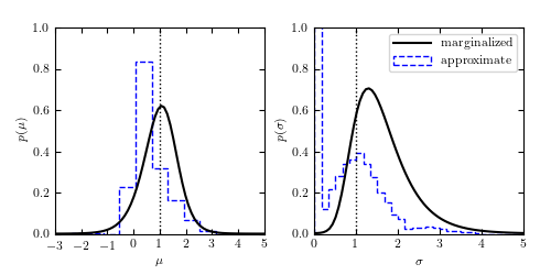
The solid lines show marginalized posterior pdfs for (left) and (right) for a Gaussian distribution with heteroscedastic Gaussian measurement errors (i.e., integrals over and for the two-dimensional distribution shown in figure 5.7). For comparison, the dashed histograms show the distributions of approximate estimates for and (the median and given by eq. 5.68, respectively) for 10,000 bootstrap resamples of the same data set. The true values of and are indicated by the vertical dotted lines.

Code output:

Python source code:

# Author: Jake VanderPlas
# License: BSD
#   The figure produced by this code is published in the textbook
#   "Statistics, Data Mining, and Machine Learning in Astronomy" (2013)
#   For more information, see http://astroML.github.com
#   To report a bug or issue, use the following forum:
#    https://groups.google.com/forum/#!forum/astroml-general
import numpy as np
from matplotlib import pyplot as plt
from astroML.stats import median_sigmaG

#----------------------------------------------------------------------
# This function adjusts matplotlib settings for a uniform feel in the textbook.
# Note that with usetex=True, fonts are rendered with LaTeX.  This may
# result in an error if LaTeX is not installed on your system.  In that case,
# you can set usetex to False.
if "setup_text_plots" not in globals():
    from astroML.plotting import setup_text_plots
setup_text_plots(fontsize=8, usetex=True)


def gaussgauss_logL(xi, ei, mu, sigma):
    """Equation 5.63: gaussian likelihood with gaussian errors"""
    ndim = len(np.broadcast(sigma, mu).shape)

    xi = xi.reshape(xi.shape + tuple(ndim * [1]))
    ei = ei.reshape(ei.shape + tuple(ndim * [1]))

    s2_e2 = sigma ** 2 + ei ** 2
    return -0.5 * np.sum(np.log(s2_e2) + (xi - mu) ** 2 / s2_e2,
                         -1 - ndim)


def approximate_mu_sigma(xi, ei, axis=None):
    """Estimates of mu0 and sigma0 via equations 5.67 - 5.68"""
    if axis is not None:
        xi = np.rollaxis(xi, axis)
        ei = np.rollaxis(ei, axis)
        axis = 0

    mu_approx, sigmaG = median_sigmaG(xi, axis=axis)
    e50 = np.median(ei, axis=axis)
    var_twiddle = (sigmaG ** 2 + ei ** 2 - e50 ** 2)
    sigma_twiddle = np.sqrt(np.maximum(0, var_twiddle))

    med = np.median(sigma_twiddle, axis=axis)
    mu = np.mean(sigma_twiddle, axis=axis)

    zeta = np.ones_like(mu)
    zeta[mu != 0] = med[mu != 0] / mu[mu != 0]

    var_approx = zeta ** 2 * sigmaG ** 2 - e50 ** 2
    sigma_approx = np.sqrt(np.maximum(0, var_approx))

    return mu_approx, sigma_approx


#--------------------------------------------------
# Generate data
np.random.seed(5)
mu_true = 1.
sigma_true = 1.
N = 10
ei = 3 * np.random.random(N)
xi = np.random.normal(mu_true, np.sqrt(sigma_true ** 2 + ei ** 2))

sigma = np.linspace(0.001, 5, 70)
mu = np.linspace(-3, 5, 70)

logL = gaussgauss_logL(xi, ei, mu, sigma[:, np.newaxis])
logL -= logL.max()
L = np.exp(logL)

p_sigma = L.sum(1)
p_sigma /= (sigma[1] - sigma[0]) * p_sigma.sum()

p_mu = L.sum(0)
p_mu /= (mu[1] - mu[0]) * p_mu.sum()

#------------------------------------------------------------
# Compute bootstrap estimates
Nbootstraps = 10000
indices = np.random.randint(0, len(xi), (len(xi), 10000))

xi_boot = xi[indices]
ei_boot = ei[indices]

mu_boot, sigma_boot = approximate_mu_sigma(xi_boot, ei_boot, 0)

#--------------------------------------------------
# Plot data
fig = plt.figure(figsize=(5, 2.5))
fig.subplots_adjust(left=0.1, right=0.95, wspace=0.24,
                    bottom=0.15, top=0.9)

# first plot the histograms for mu
ax = fig.add_subplot(121)

# plot the marginalized distribution
ax.plot(mu, p_mu, '-k', label='marginalized')

# plot the bootstrap distribution
bins = np.linspace(-3, 5, 14)
ax.hist(mu_boot, bins, histtype='step', linestyle='dashed',
        color='b', density=True, label='approximate')

# plot vertical line: newer matplotlib versions can use ax.vlines(x)
ax.plot([mu_true, mu_true], [0, 1.0], ':k', lw=1)

ax.set_xlabel(r'$\mu$')
ax.set_ylabel(r'$p(\mu)$')

ax.set_ylim(0, 1.0)


# first plot the histograms for sigma
ax = fig.add_subplot(122)

# plot the marginalized distribution
ax.plot(sigma, p_sigma, '-k', label='marginalized')

# plot the bootstrap distribution
bins = np.linspace(0, 5, 31)
ax.hist(sigma_boot, bins, histtype='step', linestyle='dashed',
        color='b', density=True, label='approximate')

# plot vertical line: newer matplotlib versions can use ax.vlines(x)
ax.plot([sigma_true, sigma_true], [0, 1.0], ':k', lw=1)

ax.set_xlabel(r'$\sigma$')
ax.set_ylabel(r'$p(\sigma)$')
ax.legend(loc=1, prop=dict(size=8))

ax.set_xlim(0, 5.0)
ax.set_ylim(0, 1.0)

plt.show()

[download source: fig_posterior_gaussgauss.py]