Poisson Statistics with arbitrarily small bins

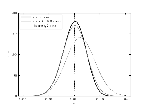
Figure 5.16

The comparison of the continuous method (figure 5.14) and the binned method (figure 5.15) on the same data set. In the limit of a large number of bins, most bins register only zero or one count, and the binned Poisson statistic gives nearly the same marginalized distribution for a as the continuous statistic. For as few as two bins, the constraint on the slope is only slightly biased.

Code output:

Python source code:

# Author: Jake VanderPlas
# License: BSD
#   The figure produced by this code is published in the textbook
#   "Statistics, Data Mining, and Machine Learning in Astronomy" (2013)
#   For more information, see http://astroML.github.com
#   To report a bug or issue, use the following forum:
#    https://groups.google.com/forum/#!forum/astroml-general
import numpy as np
from matplotlib import pyplot as plt
from astroML.stats.random import linear

#----------------------------------------------------------------------
# This function adjusts matplotlib settings for a uniform feel in the textbook.
# Note that with usetex=True, fonts are rendered with LaTeX.  This may
# result in an error if LaTeX is not installed on your system.  In that case,
# you can set usetex to False.
if "setup_text_plots" not in globals():
    from astroML.plotting import setup_text_plots
setup_text_plots(fontsize=8, usetex=True)


def logL_continuous(x, a, xmin, xmax):
    """Continuous log-likelihood (Eq. 5.84)"""
    x = x.ravel()
    a = a.reshape(a.shape + (1,))

    mu = 0.5 * (xmin + xmax)
    W = (xmax - xmin)

    return np.sum(np.log(a * (x - mu) + 1. / W), -1)


def logL_poisson(xi, yi, a, b):
    """poisson log-likelihood (Eq. 5.88)"""
    xi = xi.ravel()
    yi = yi.ravel()
    a = a.reshape(a.shape + (1,))
    b = b.reshape(b.shape + (1,))
    yyi = a * xi + b
    return np.sum(yi * np.log(yyi) - yyi, -1)

#----------------------------------------------------------------------
# draw the data
np.random.seed(0)
N = 200
a_true = 0.01
xmin = 0.0
xmax = 10.0

lin_dist = linear(xmin, xmax, a_true)
x = lin_dist.rvs(N)

a = np.linspace(0.0, 0.02, 101)
b = np.linspace(0.00001, 0.15, 51)

#------------------------------------------------------------
# Compute the log-likelihoods

# continuous case
logL = logL_continuous(x, a, xmin, xmax)
L_c = np.exp(logL - logL.max())
L_c /= L_c.sum() * (a[1] - a[0])

# discrete case: compute for 2 and 1000 bins
nbins = [1000, 2]
L_p = [0, 0]

for i, n in enumerate(nbins):
    yi, bins = np.histogram(x, bins=np.linspace(xmin, xmax, n + 1))
    xi = 0.5 * (bins[:-1] + bins[1:])

    factor = N * (xmax - xmin) * 1. / n

    logL = logL_poisson(xi, yi, factor * a, factor * b[:, None])
    L_p[i] = np.exp(logL - np.max(logL)).sum(0)
    L_p[i] /= L_p[i].sum() * (a[1] - a[0])


#------------------------------------------------------------
# Plot the results
fig, ax = plt.subplots(figsize=(5, 3.75))

ax.plot(a, L_c, '-k', label='continuous')
for L, ls, n in zip(L_p, ['-', '--'], nbins):
    ax.plot(a, L, ls, color='gray', lw=1,
            label='discrete, %i bins' % n)

# plot a vertical line: in newer matplotlib, use ax.vlines([a_true])
ylim = (0, 200)
ax.plot([a_true, a_true], ylim, ':k', lw=1)

ax.set_xlim(-0.001, 0.021)
ax.set_ylim(ylim)

ax.set_xlabel('$a$')
ax.set_ylabel('$p(a)$')

ax.legend(loc=2)

plt.show()

[download source: fig_poisson_comparison.py]