Eddington-Malmquist & Lutz-Kelker Biases

Figure 5.3

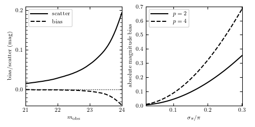
An illustration of the Eddington-Malmquist (left) and Lutz-Kelker (right) biases for mock data sets that simulate upcoming LSST and Gaia surveys (see text). The left panel shows a bias in photometric calibration when using pairs of measurements of the same stars with realistic photometric error distributions. Depending on the adopted faint limit (x-axis), the median difference between two measurements (dashed line) is biased when this limit is too close to the 5-sigma data limit (corresponding to errors of 0.2 mag); in this example the 5-sigma magnitude limit is set to 24. The solid line shows the assumed random measurement errors - if the number of stars in the sample is large, the random error for magnitude difference may become much smaller than the bias. The right panel shows the bias in absolute magnitude for samples calibrated using trigonometric parallax measurements with relative errors , and two hypothetical parallax distributions given by eq. 5.41 and p = 2, 4.

Code output:

Python source code:

# Author: Jake VanderPlas
# License: BSD
#   The figure produced by this code is published in the textbook
#   "Statistics, Data Mining, and Machine Learning in Astronomy" (2013)
#   For more information, see http://astroML.github.com
#   To report a bug or issue, use the following forum:
#    https://groups.google.com/forum/#!forum/astroml-general
import numpy as np
from matplotlib import pyplot as plt
from astroML.stats import median_sigmaG

#----------------------------------------------------------------------
# This function adjusts matplotlib settings for a uniform feel in the textbook.
# Note that with usetex=True, fonts are rendered with LaTeX.  This may
# result in an error if LaTeX is not installed on your system.  In that case,
# you can set usetex to False.
if "setup_text_plots" not in globals():
    from astroML.plotting import setup_text_plots
setup_text_plots(fontsize=8, usetex=True)


def generate_magnitudes(N, k=0.6, m_min=20, m_max=25):
    """
    generate magnitudes from a distribution with
      p(m) ~ 10^(k m)
    """
    klog10 = k * np.log(10)
    Pmin = np.exp(klog10 * m_min)
    Pmax = np.exp(klog10 * m_max)
    return (1. / klog10) * np.log(Pmin + (Pmax - Pmin) * np.random.random(N))


def mag_errors(m_true, m5=24.0, fGamma=0.039):
    """
    compute magnitude errors based on the true magnitude and the
    5-sigma limiting magnitude, m5
    """
    x = 10 ** (0.4 * (mtrue - m5))
    return np.sqrt((0.04 - fGamma) * x + fGamma * x ** 2)

#----------------------------------------------------------------------
# Compute the Eddington-Malmquist bias & scatter
np.random.seed(42)

mtrue = generate_magnitudes(int(1E6), m_min=20, m_max=25)
photomErr = mag_errors(mtrue)

m1 = mtrue + np.random.normal(0, photomErr)
m2 = mtrue + np.random.normal(0, photomErr)
dm = m1 - m2

mGrid = np.linspace(21, 24, 50)
medGrid = np.zeros(mGrid.size)
sigGrid = np.zeros(mGrid.size)

for i in range(mGrid.size):
    medGrid[i], sigGrid[i] = median_sigmaG(dm[m1 < mGrid[i]])

#----------------------------------------------------------------------
# Lutz-Kelker bias and scatter

mtrue = generate_magnitudes(int(1E6), m_min=17, m_max=20)
relErr = 0.3 * 10 ** (0.4 * (mtrue - 20))

pErrGrid = np.arange(0.02, 0.31, 0.01)

deltaM2 = 5 * np.log(1 + 2 * relErr ** 2)
deltaM4 = 5 * np.log(1 + 4 * relErr ** 2)

med2 = [np.median(deltaM2[relErr < e]) for e in pErrGrid]
med4 = [np.median(deltaM4[relErr < e]) for e in pErrGrid]

#----------------------------------------------------------------------
# plot results
fig = plt.figure(figsize=(5, 2.5))
fig.subplots_adjust(left=0.1, right=0.95, wspace=0.25,
                    bottom=0.17, top=0.95)

ax = fig.add_subplot(121)
ax.plot(mGrid, sigGrid, '-k', label='scatter')
ax.plot(mGrid, medGrid, '--k', label='bias')
ax.plot(mGrid, 0 * mGrid, ':k', lw=1)
ax.legend(loc=2)

ax.set_xlabel(r'$m_{\rm obs}$')
ax.set_ylabel('bias/scatter (mag)')

ax.set_ylim(-0.04, 0.21)
ax.xaxis.set_major_locator(plt.MultipleLocator(1.0))
ax.yaxis.set_major_locator(plt.MultipleLocator(0.1))
ax.yaxis.set_minor_locator(plt.MultipleLocator(0.01))

for l in ax.yaxis.get_minorticklines():
    l.set_markersize(3)

ax = fig.add_subplot(122)
ax.plot(pErrGrid, med2, '-k', label='$p=2$')
ax.plot(pErrGrid, med4, '--k', label='$p=4$')
ax.legend(loc=2)
ax.set_xlabel(r'$\sigma_\pi / \pi$')
ax.set_ylabel('absolute magnitude bias')
ax.xaxis.set_major_locator(plt.MultipleLocator(0.1))
ax.set_xlim(0.02, 0.301)
ax.set_ylim(0, 0.701)

plt.show()

[download source: fig_lutz_kelker.py]