Log-likelihood for Cauchy Distribution

Figure 5.10

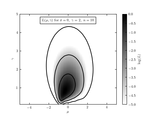
An illustration of the logarithm of posterior probability distribution for and , (see eq. 5.75) for N = 10 (the sample is generated using the Cauchy distribution with and ). The maximum of L is renormalized to 0, and color coded as shown in the legend. The contours enclose the regions that contain 0.683, 0.955 and 0.997 of the cumulative (integrated) posterior probability.

Code output:

mu from likelihood: [-0.36231884]
gamma from likelihood: [0.81014493]

mu from median -0.2625695623133895
gamma from quartiles: 1.10950042396172

Python source code:

# Author: Jake VanderPlas
# License: BSD
#   The figure produced by this code is published in the textbook
#   "Statistics, Data Mining, and Machine Learning in Astronomy" (2013)
#   For more information, see http://astroML.github.com
#   To report a bug or issue, use the following forum:
#    https://groups.google.com/forum/#!forum/astroml-general
from __future__ import print_function, division

import numpy as np
from matplotlib import pyplot as plt
from scipy.stats import cauchy
from astroML.plotting.mcmc import convert_to_stdev
from astroML.stats import median_sigmaG

#----------------------------------------------------------------------
# This function adjusts matplotlib settings for a uniform feel in the textbook.
# Note that with usetex=True, fonts are rendered with LaTeX.  This may
# result in an error if LaTeX is not installed on your system.  In that case,
# you can set usetex to False.
if "setup_text_plots" not in globals():
    from astroML.plotting import setup_text_plots
setup_text_plots(fontsize=8, usetex=True)


def cauchy_logL(xi, gamma, mu):
    """Equation 5.74: cauchy likelihood"""
    xi = np.asarray(xi)
    n = xi.size
    shape = np.broadcast(gamma, mu).shape

    xi = xi.reshape(xi.shape + tuple([1 for s in shape]))

    return ((n - 1) * np.log(gamma)
            - np.sum(np.log(gamma ** 2 + (xi - mu) ** 2), 0))


#------------------------------------------------------------
# Define the grid and compute logL
gamma = np.linspace(0.1, 5, 70)
mu = np.linspace(-5, 5, 70)

np.random.seed(44)
mu0 = 0
gamma0 = 2
xi = cauchy(mu0, gamma0).rvs(10)

logL = cauchy_logL(xi, gamma[:, np.newaxis], mu)
logL -= logL.max()

#------------------------------------------------------------
# Find the max and print some information
i, j = np.where(logL >= np.max(logL))

print("mu from likelihood:", mu[j])
print("gamma from likelihood:", gamma[i])
print()

med, sigG = median_sigmaG(xi)
print("mu from median", med)
print("gamma from quartiles:", sigG / 1.483)  # Equation 3.54
print()

#------------------------------------------------------------
# Plot the results
fig = plt.figure(figsize=(5, 3.75))
plt.imshow(logL, origin='lower', cmap=plt.cm.binary,
           extent=(mu[0], mu[-1], gamma[0], gamma[-1]),
           aspect='auto')
plt.colorbar().set_label(r'$\log(L)$')
plt.clim(-5, 0)

plt.contour(mu, gamma, convert_to_stdev(logL),
            levels=(0.683, 0.955, 0.997),
            colors='k')

plt.text(0.5, 0.93,
         r'$L(\mu,\gamma)\ \mathrm{for}\ \bar{x}=0,\ \gamma=2,\ n=10$',
         bbox=dict(ec='k', fc='w', alpha=0.9),
         ha='center', va='center', transform=plt.gca().transAxes)

plt.xlabel(r'$\mu$')
plt.ylabel(r'$\gamma$')

plt.show()

[download source: fig_likelihood_cauchy.py]