Selection of Histogram bin size

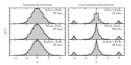
Figure 5.20

The results of Scott’s rule, the Freedman-Diaconis rule, and Knuth’s rule for selecting the optimal bin width for a histogram. These histograms are based on 5000 points drawn from the shown pdfs. On the left is a simple normal distribution. On the right is a Laplacian distribution at the center, with two small Gaussian peaks added in the wings.

Code output:

Python source code:

# Author: Jake VanderPlas
# License: BSD
#   The figure produced by this code is published in the textbook
#   "Statistics, Data Mining, and Machine Learning in Astronomy" (2013)
#   For more information, see http://astroML.github.com
#   To report a bug or issue, use the following forum:
#    https://groups.google.com/forum/#!forum/astroml-general
import numpy as np
from matplotlib import pyplot as plt
from scipy import stats
from astropy.visualization import hist

#----------------------------------------------------------------------
# This function adjusts matplotlib settings for a uniform feel in the textbook.
# Note that with usetex=True, fonts are rendered with LaTeX.  This may
# result in an error if LaTeX is not installed on your system.  In that case,
# you can set usetex to False.
if "setup_text_plots" not in globals():
    from astroML.plotting import setup_text_plots
setup_text_plots(fontsize=8, usetex=True)


def plot_labeled_histogram(style, data, name,
                           x, pdf_true, ax=None,
                           hide_x=False,
                           hide_y=False):
    if ax is not None:
        ax = plt.axes(ax)

    counts, bins, patches = hist(data, bins=style, ax=ax,
                                 color='k', histtype='step', density=True)
    ax.text(0.95, 0.93, '%s:\n%i bins' % (name, len(counts)),
            transform=ax.transAxes,
            ha='right', va='top')

    ax.fill(x, pdf_true, '-', color='#CCCCCC', zorder=0)

    if hide_x:
        ax.xaxis.set_major_formatter(plt.NullFormatter())
    if hide_y:
        ax.yaxis.set_major_formatter(plt.NullFormatter())

    ax.set_xlim(-5, 5)

    return ax


#------------------------------------------------------------
# Set up distributions:
Npts = 5000
np.random.seed(0)
x = np.linspace(-6, 6, 1000)

# Gaussian distribution
data_G = stats.norm(0, 1).rvs(Npts)
pdf_G = stats.norm(0, 1).pdf(x)

# Non-Gaussian distribution
distributions = [stats.laplace(0, 0.4),
                 stats.norm(-4.0, 0.2),
                 stats.norm(4.0, 0.2)]

weights = np.array([0.8, 0.1, 0.1])
weights /= weights.sum()

data_NG = np.hstack(d.rvs(int(w * Npts))
                    for (d, w) in zip(distributions, weights))
pdf_NG = sum(w * d.pdf(x)
             for (d, w) in zip(distributions, weights))

#------------------------------------------------------------
# Plot results
fig = plt.figure(figsize=(5, 2.5))
fig.subplots_adjust(hspace=0, left=0.07, right=0.95, wspace=0.05, bottom=0.15)
ax = [fig.add_subplot(3, 2, i + 1) for i in range(6)]

# first column: Gaussian distribution
plot_labeled_histogram('scott', data_G, 'Scott\'s Rule', x, pdf_G,
                       ax=ax[0], hide_x=True, hide_y=True)
plot_labeled_histogram('freedman', data_G, 'Freed.-Diac.', x, pdf_G,
                       ax=ax[2], hide_x=True, hide_y=True)
plot_labeled_histogram('knuth', data_G, 'Knuth\'s Rule', x, pdf_G,
                       ax=ax[4], hide_x=False, hide_y=True)

ax[0].set_title('Gaussian distribution')
ax[2].set_ylabel('$p(x)$')
ax[4].set_xlabel('$x$')

# second column: non-gaussian distribution
plot_labeled_histogram('scott', data_NG, 'Scott\'s Rule', x, pdf_NG,
                       ax=ax[1], hide_x=True, hide_y=True)
plot_labeled_histogram('freedman', data_NG, 'Freed.-Diac.', x, pdf_NG,
                       ax=ax[3], hide_x=True, hide_y=True)
plot_labeled_histogram('knuth', data_NG, 'Knuth\'s Rule', x, pdf_NG,
                       ax=ax[5], hide_x=False, hide_y=True)

ax[1].set_title('non-Gaussian distribution')
ax[5].set_xlabel('$x$')

plt.show()

[download source: fig_hist_binsize.py]