MCMC for the Cauchy distribution

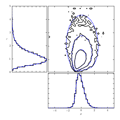
Figure 5.22

Markov chain monte carlo (MCMC) estimates of the posterior pdf for parameters describing the Cauchy distribution. The data are the same as those used in figure 5.10: the dashed curves in the top-right panel show the results of direct computation on a regular grid from that diagram. The solid curves are the corresponding MCMC estimates using 10,000 sample points. The left and the bottom panels show marginalized distributions.

Code output:

Python source code:

# Author: Jake VanderPlas (adapted to PyMC3 by Brigitta Sipocz)
# License: BSD
#   The figure produced by this code is published in the textbook
#   "Statistics, Data Mining, and Machine Learning in Astronomy" (2013)
#   For more information, see http://astroML.github.com
#   To report a bug or issue, use the following forum:
#    https://groups.google.com/forum/#!forum/astroml-general
import numpy as np
from scipy.stats import cauchy
from matplotlib import pyplot as plt
from astroML.plotting.mcmc import convert_to_stdev

import pymc3 as pm

# ----------------------------------------------------------------------
# This function adjusts matplotlib settings for a uniform feel in the textbook.
# Note that with usetex=True, fonts are rendered with LaTeX.  This may
# result in an error if LaTeX is not installed on your system.  In that case,
# you can set usetex to False.
if "setup_text_plots" not in globals():
    from astroML.plotting import setup_text_plots
setup_text_plots(fontsize=8, usetex=True)


def cauchy_logL(xi, sigma, mu):
    """Equation 5.74: cauchy likelihood"""
    xi = np.asarray(xi)
    n = xi.size
    shape = np.broadcast(sigma, mu).shape

    xi = xi.reshape(xi.shape + tuple([1 for s in shape]))

    return ((n - 1) * np.log(sigma)
            - np.sum(np.log(sigma ** 2 + (xi - mu) ** 2), 0))


# ----------------------------------------------------------------------
# Draw the sample from a Cauchy distribution
np.random.seed(44)
mu_0 = 0
gamma_0 = 2
xi = cauchy(mu_0, gamma_0).rvs(10)

# ----------------------------------------------------------------------
# Set up and run MCMC:
with pm.Model():
    mu = pm.Uniform('mu', -5, 5)
    log_gamma = pm.Uniform('log_gamma', -10, 10)

    # set up our observed variable x
    x = pm.Cauchy('x', mu, np.exp(log_gamma), observed=xi)

    trace = pm.sample(draws=12000, tune=1000, cores=1)

# compute histogram of results to plot below
L_MCMC, mu_bins, gamma_bins = np.histogram2d(trace['mu'],
                                             np.exp(trace['log_gamma']),
                                             bins=(np.linspace(-5, 5, 41),
                                                   np.linspace(0, 5, 41)))
L_MCMC[L_MCMC == 0] = 1E-16  # prevents zero-division errors

# ----------------------------------------------------------------------
# Compute likelihood analytically for comparison
mu = np.linspace(-5, 5, 70)
gamma = np.linspace(0.1, 5, 70)
logL = cauchy_logL(xi, gamma[:, np.newaxis], mu)
logL -= logL.max()

p_mu = np.exp(logL).sum(0)
p_mu /= p_mu.sum() * (mu[1] - mu[0])

p_gamma = np.exp(logL).sum(1)
p_gamma /= p_gamma.sum() * (gamma[1] - gamma[0])

hist_mu, bins_mu = np.histogram(trace['mu'], bins=mu_bins, density=True)
hist_gamma, bins_gamma = np.histogram(np.exp(trace['log_gamma']),
                                      bins=gamma_bins, density=True)


# ----------------------------------------------------------------------
# plot the results
fig = plt.figure(figsize=(5, 5))

# first axis: likelihood contours
ax1 = fig.add_axes((0.4, 0.4, 0.55, 0.55))
ax1.xaxis.set_major_formatter(plt.NullFormatter())
ax1.yaxis.set_major_formatter(plt.NullFormatter())

ax1.contour(mu, gamma, convert_to_stdev(logL),
            levels=(0.683, 0.955, 0.997),
            colors='b', linestyles='dashed')

ax1.contour(0.5 * (mu_bins[:-1] + mu_bins[1:]),
            0.5 * (gamma_bins[:-1] + gamma_bins[1:]),
            convert_to_stdev(np.log(L_MCMC.T)),
            levels=(0.683, 0.955, 0.997),
            colors='k')

# second axis: marginalized over mu
ax2 = fig.add_axes((0.1, 0.4, 0.29, 0.55))
ax2.xaxis.set_major_formatter(plt.NullFormatter())
ax2.plot(hist_gamma, 0.5 * (bins_gamma[1:] + bins_gamma[:-1]
                            - bins_gamma[1] + bins_gamma[0]),
         '-k', drawstyle='steps')
ax2.plot(p_gamma, gamma, '--b')
ax2.set_ylabel(r'$\gamma$')
ax2.set_ylim(0, 5)

# third axis: marginalized over gamma
ax3 = fig.add_axes((0.4, 0.1, 0.55, 0.29))
ax3.yaxis.set_major_formatter(plt.NullFormatter())
ax3.plot(0.5 * (bins_mu[1:] + bins_mu[:-1]), hist_mu,
         '-k', drawstyle='steps-mid')
ax3.plot(mu, p_mu, '--b')
ax3.set_xlabel(r'$\mu$')
plt.xlim(-5, 5)

plt.show()

[download source: fig_cauchy_mcmc.py]