Kurtosis and Skew
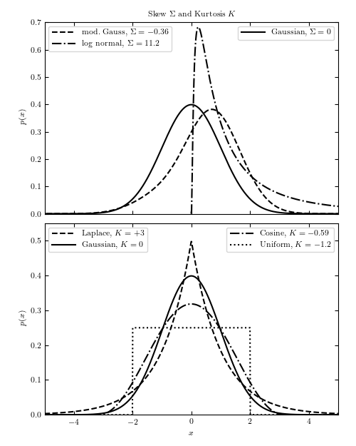
Figure 3.6.
An example of distributions with different skewness
 (top panel) and kurtosis K (bottom panel). The modified
Gaussian in the upper panel is a normal distribution multiplied by a
Gram-Charlier series (see eq. 4.70), with a0 = 2, a1 = 1, and a2 = 0.5.
The log-normal has
(top panel) and kurtosis K (bottom panel). The modified
Gaussian in the upper panel is a normal distribution multiplied by a
Gram-Charlier series (see eq. 4.70), with a0 = 2, a1 = 1, and a2 = 0.5.
The log-normal has  .
.
# Author: Jake VanderPlas
# License: BSD
#   The figure produced by this code is published in the textbook
#   "Statistics, Data Mining, and Machine Learning in Astronomy" (2013)
#   For more information, see http://astroML.github.com
#   To report a bug or issue, use the following forum:
#    https://groups.google.com/forum/#!forum/astroml-general
import numpy as np
from scipy import stats
from matplotlib import pyplot as plt

#----------------------------------------------------------------------
# This function adjusts matplotlib settings for a uniform feel in the textbook.
# Note that with usetex=True, fonts are rendered with LaTeX.  This may
# result in an error if LaTeX is not installed on your system.  In that case,
# you can set usetex to False.
if "setup_text_plots" not in globals():
    from astroML.plotting import setup_text_plots
setup_text_plots(fontsize=8, usetex=True)

fig = plt.figure(figsize=(5, 6.25))
fig.subplots_adjust(right=0.95, hspace=0.05, bottom=0.07, top=0.95)

# First show distributions with different skeq
ax = fig.add_subplot(211)
x = np.linspace(-8, 8, 1000)
N = stats.norm(0, 1)

l1, = ax.plot(x, N.pdf(x), '-k',
              label=r'${\rm Gaussian,}\ \Sigma=0$')

l2, = ax.plot(x, 0.5 * N.pdf(x) * (2 + x + 0.5 * (x * x - 1)),
              '--k', label=r'${\rm mod.\ Gauss,}\ \Sigma=-0.36$')
l3, = ax.plot(x[499:], stats.lognorm(1.2).pdf(x[499:]), '-.k',
              label=r'$\rm log\ normal,\ \Sigma=11.2$')

ax.set_xlim(-5, 5)
ax.set_ylim(0, 0.7001)
ax.set_ylabel('$p(x)$')
ax.xaxis.set_major_formatter(plt.NullFormatter())

# trick to show multiple legends
leg1 = ax.legend([l1], [l1.get_label()], loc=1)
leg2 = ax.legend([l2, l3], (l2.get_label(), l3.get_label()), loc=2)
ax.add_artist(leg1)
ax.set_title('Skew $\Sigma$ and Kurtosis $K$')

# next show distributions with different kurtosis
ax = fig.add_subplot(212)
x = np.linspace(-5, 5, 1000)
l1, = ax.plot(x, stats.laplace(0, 1).pdf(x), '--k',
              label=r'${\rm Laplace,}\ K=+3$')
l2, = ax.plot(x, stats.norm(0, 1).pdf(x), '-k',
              label=r'${\rm Gaussian,}\ K=0$')
l3, = ax.plot(x, stats.cosine(0, 1).pdf(x), '-.k',
              label=r'${\rm Cosine,}\ K=-0.59$')
l4, = ax.plot(x, stats.uniform(-2, 4).pdf(x), ':k',
              label=r'${\rm Uniform,}\ K=-1.2$')

ax.set_xlim(-5, 5)
ax.set_ylim(0, 0.55)
ax.set_xlabel('$x$')
ax.set_ylabel('$p(x)$')

# trick to show multiple legends
leg1 = ax.legend((l1, l2), (l1.get_label(), l2.get_label()), loc=2)
leg2 = ax.legend((l3, l4), (l3.get_label(), l4.get_label()), loc=1)
ax.add_artist(leg1)

plt.show()