Correlation estimates

Figure 3.24.

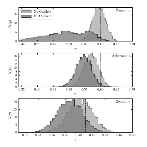
Bootstrap estimates of the distribution of Pearson’s, Spearman’s, and Kendall’s correlation coefficients based on 2000 resamplings of the 1000 points shown in figure 3.23. The true values are shown by the dashed lines. It is clear that Pearson’s correlation coefficient is not robust to contamination.

Code output:

@pickle_results: computing results and saving to 'fig_correlations_dump.pkl'

Python source code:

# Author: Jake VanderPlas
# License: BSD
#   The figure produced by this code is published in the textbook
#   "Statistics, Data Mining, and Machine Learning in Astronomy" (2013)
#   For more information, see http://astroML.github.com
#   To report a bug or issue, use the following forum:
#    https://groups.google.com/forum/#!forum/astroml-general
import numpy as np
from scipy import stats
from matplotlib import pyplot as plt

from astroML.stats.random import bivariate_normal
from astroML.utils.decorators import pickle_results

# percent sign must be escaped if usetex=True
import matplotlib
if matplotlib.rcParams.get('text.usetex'):
    pct = '\%'
else:
    pct = '%'

#----------------------------------------------------------------------
# This function adjusts matplotlib settings for a uniform feel in the textbook.
# Note that with usetex=True, fonts are rendered with LaTeX.  This may
# result in an error if LaTeX is not installed on your system.  In that case,
# you can set usetex to False.
if "setup_text_plots" not in globals():
    from astroML.plotting import setup_text_plots
setup_text_plots(fontsize=8, usetex=True)

#------------------------------------------------------------
# Set parameters for the distributions
Nbootstraps = 5000
N = 1000

sigma1 = 2.0
sigma2 = 1.0
mu = (10.0, 10.0)
alpha_deg = 45.0
alpha = alpha_deg * np.pi / 180
f = 0.01

#------------------------------------------------------------
# sample the distribution
# without outliers and with outliers
np.random.seed(0)
X = bivariate_normal(mu, sigma1, sigma2, alpha, N)

X_out = X.copy()
X_out[:int(f * N)] = bivariate_normal(mu, 2, 5,
                                      45 * np.pi / 180., int(f * N))

# true values of rho (pearson/spearman r) and tau
# tau value comes from Eq. 41 of arXiv:1011.2009
rho_true = 0.6
tau_true = 2 / np.pi * np.arcsin(rho_true)


#------------------------------------------------------------
# Create a function to compute the statistics.  Since this
#  takes a while, we'll use the "pickle_results" decorator
#  to save the results of the computation to disk
@pickle_results('fig_correlations_dump.pkl')
def compute_results(N, Nbootstraps):
    results = np.zeros((3, 2, Nbootstraps))

    for k in range(Nbootstraps):
        ind = np.random.randint(N, size=N)
        for j, data in enumerate([X, X_out]):
            x = data[ind, 0]
            y = data[ind, 1]
            for i, statistic in enumerate([stats.pearsonr,
                                           stats.spearmanr,
                                           stats.kendalltau]):
                results[i, j, k] = statistic(x, y)[0]

    return results

results = compute_results(N, Nbootstraps)

#------------------------------------------------------------
# Plot the results in a three-panel plot
fig = plt.figure(figsize=(5, 5))
fig.subplots_adjust(bottom=0.1, top=0.95, hspace=0.35)

histargs = (dict(alpha=0.5, label='No Outliers'),
            dict(alpha=0.8, label='%i%s Outliers' % (int(f * 100), pct)))

distributions = ['Pearson-r', 'Spearman-r', r'Kendall-$\tau$']
xlabels = ['r_p', 'r_s', r'\tau']\

for i in range(3):
    ax = fig.add_subplot(311 + i)
    for j in range(2):
        ax.hist(results[i, j], 40, histtype='stepfilled', fc='gray',
                density=True, **histargs[j])

    if i == 0:
        ax.legend(loc=2)

    ylim = ax.get_ylim()
    if i < 2:
        ax.plot([rho_true, rho_true], ylim, '--k', lw=1)
        ax.set_xlim(0.34, 0.701)
    else:
        ax.plot([tau_true, tau_true], ylim, '--k', lw=1)
        ax.set_xlim(0.31, 0.48)
    ax.set_ylim(ylim)

    ax.text(0.98, 0.95, distributions[i], ha='right', va='top',
            transform=ax.transAxes)

    ax.set_xlabel('$%s$' % xlabels[i])
    ax.set_ylabel('$N(%s)$' % xlabels[i])

plt.show()

[download source: fig_correlations.py]