Minimum component fitting procedure
Figure 10.12
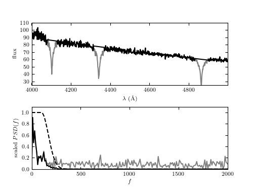
The intermediate steps of the minimum component filter procedure applied to the spectrum of a white dwarf from the SDSS data set (mjd= 52199, plate=659, fiber=381). The top panel shows the input spectrum; the masked sections of the input spectrum are shown by thin lines (i.e., step 1 of the process in Section 10.2.5). The bottom panel shows the PSD of the masked spectrum, after the linear fit has been subtracted (gray line). A simple low-pass filter (dashed line) is applied, and the resulting filtered spectrum (dark line) is used to construct the result shown in figure 10.13.
Minimum component filtering is explained in Wall & Jenkins, as well as Wall 1997, A&A 122:371. The minimum component algorithm is implemented in astroML.filters.min_component_filter
Downloading http://das.sdss.org/spectro/1d_26/0659/1d/spSpec-52199-0659-381.fit
[=                                      ]  4.6kb / 182.8kb
[==                                     ]  9.1kb / 182.8kb
[===                                    ]  13.7kb / 182.8kb
[====                                   ]  18.3kb / 182.8kb
[=====                                  ]  22.9kb / 182.8kb
[======                                 ]  27.4kb / 182.8kb
[=======                                ]  32.0kb / 182.8kb
[========                               ]  36.6kb / 182.8kb
[=========                              ]  41.1kb / 182.8kb
[==========                             ]  45.7kb / 182.8kb
[===========                            ]  50.3kb / 182.8kb
[============                           ]  54.8kb / 182.8kb
[=============                          ]  59.4kb / 182.8kb
[==============                         ]  64.0kb / 182.8kb
[===============                        ]  68.6kb / 182.8kb
[================                       ]  73.1kb / 182.8kb
[=================                      ]  77.7kb / 182.8kb
[==================                     ]  82.3kb / 182.8kb
[===================                    ]  86.8kb / 182.8kb
[====================                   ]  91.4kb / 182.8kb
[=====================                  ]  96.0kb / 182.8kb
[======================                 ]  100.5kb / 182.8kb
[=======================                ]  105.1kb / 182.8kb
[========================               ]  109.7kb / 182.8kb
[=========================              ]  114.3kb / 182.8kb
[==========================             ]  118.8kb / 182.8kb
[===========================            ]  123.4kb / 182.8kb
[============================           ]  128.0kb / 182.8kb
[=============================          ]  132.5kb / 182.8kb
[==============================         ]  137.1kb / 182.8kb
[===============================        ]  141.7kb / 182.8kb
[================================       ]  146.2kb / 182.8kb
[=================================      ]  150.8kb / 182.8kb
[==================================     ]  155.4kb / 182.8kb
[===================================    ]  160.0kb / 182.8kb
[====================================   ]  164.5kb / 182.8kb
[=====================================  ]  169.1kb / 182.8kb
[====================================== ]  173.7kb / 182.8kb
[=======================================]  178.2kb / 182.8kb
[========================================]  182.8kb / 182.8kb
caching to /Users/bsipocz/astroML_data/SDSSspec/0659/spSpec-52199-0659-381.fit
# Author: Jake VanderPlas
# License: BSD
#   The figure produced by this code is published in the textbook
#   "Statistics, Data Mining, and Machine Learning in Astronomy" (2013)
#   For more information, see http://astroML.github.com
#   To report a bug or issue, use the following forum:
#    https://groups.google.com/forum/#!forum/astroml-general
import numpy as np
from matplotlib import pyplot as plt

from scipy import fftpack

from astroML.fourier import PSD_continuous
from astroML.datasets import fetch_sdss_spectrum

#----------------------------------------------------------------------
# This function adjusts matplotlib settings for a uniform feel in the textbook.
# Note that with usetex=True, fonts are rendered with LaTeX.  This may
# result in an error if LaTeX is not installed on your system.  In that case,
# you can set usetex to False.
if "setup_text_plots" not in globals():
    from astroML.plotting import setup_text_plots
setup_text_plots(fontsize=8, usetex=True)

#------------------------------------------------------------
# Fetch the spectrum from SDSS database & pre-process
plate = 659
mjd = 52199
fiber = 381

data = fetch_sdss_spectrum(plate, mjd, fiber)

lam = data.wavelength()
spec = data.spectrum

# wavelengths are logorithmically spaced: we'll work in log(lam)
loglam = np.log10(lam)

flag = (lam > 4000) & (lam < 5000)
lam = lam[flag]
loglam = loglam[flag]
spec = spec[flag]

lam = lam[:-1]
loglam = loglam[:-1]
spec = spec[:-1]

#----------------------------------------------------------------------
# First step: mask-out significant features
feature_mask = (((lam > 4080) & (lam < 4130)) |
                ((lam > 4315) & (lam < 4370)) |
                ((lam > 4830) & (lam < 4900)))

#----------------------------------------------------------------------
# Second step: fit a line to the unmasked portion of the spectrum
XX = loglam[:, None] ** np.arange(2)
beta = np.linalg.lstsq(XX[~feature_mask], spec[~feature_mask])[0]

spec_fit = np.dot(XX, beta)
spec_patched = spec - spec_fit
spec_patched[feature_mask] = 0

#----------------------------------------------------------------------
# Third step: Fourier transform the patched spectrum
N = len(loglam)
df = 1. / N / (loglam[1] - loglam[0])
f = fftpack.ifftshift(df * (np.arange(N) - N / 2.))
spec_patched_FT = fftpack.fft(spec_patched)

#----------------------------------------------------------------------
# Fourth step: Low-pass filter on the transform
filt = np.exp(- (0.01 * (abs(f) - 100.)) ** 2)
filt[abs(f) < 100] = 1

spec_filt_FT = spec_patched_FT * filt

#----------------------------------------------------------------------
# Fifth step: inverse Fourier transform, and add back the fit
spec_filt = fftpack.ifft(spec_filt_FT)
spec_filt += spec_fit

#----------------------------------------------------------------------
# plot results
fig = plt.figure(figsize=(5, 3.75))
fig.subplots_adjust(hspace=0.35)

ax = fig.add_subplot(211)
ax.plot(lam, spec, '-', c='gray')
ax.plot(lam, spec_patched + spec_fit, '-k')

ax.set_ylim(25, 110)

ax.set_xlabel(r'$\lambda\ {\rm(\AA)}$')
ax.set_ylabel('flux')

ax = fig.add_subplot(212)
factor = 15 * (loglam[1] - loglam[0])
ax.plot(fftpack.fftshift(f),
        factor * fftpack.fftshift(abs(spec_patched_FT) ** 1),
        '-', c='gray', label='masked/shifted spectrum')
ax.plot(fftpack.fftshift(f),
        factor * fftpack.fftshift(abs(spec_filt_FT) ** 1),
        '-k', label='filtered spectrum')
ax.plot(fftpack.fftshift(f),
        fftpack.fftshift(filt), '--k', label='filter')

ax.set_xlim(0, 2000)
ax.set_ylim(0, 1.1)

ax.set_xlabel('$f$')
ax.set_ylabel('scaled $PSD(f)$')

plt.show()