Fast Fourier Transform Example

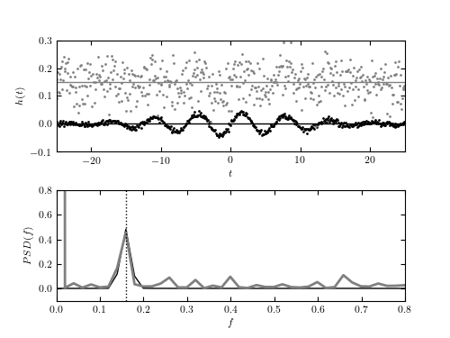
Figure 10.5

The discrete Fourier transform (bottom panel) for two noisy data sets shown in the top panel. For 512 evenly sampled times t (dt = 0.977), points are drawn from h(t) = a + sin(t)G(t), where G(t) is a Gaussian N(mu = 0,sigma = 10). Gaussian noise with sigma = 0.05 (top data set) and 0.005 (bottom data set) is added to signal h(t). The value of the offset a is 0.15 and 0, respectively. The discrete Fourier transform is computed as described in Section 10.2.3. For both noise realizations, the correct frequency f = (2pi)-1 ~ 0.159 is easily discernible in the bottom panel. Note that the height of peaks is the same for both noise realizations. The large value of abs(H(f = 0)) for data with larger noise is due to the vertical offset.

Code output:

Python source code:

# Author: Jake VanderPlas
# License: BSD
#   The figure produced by this code is published in the textbook
#   "Statistics, Data Mining, and Machine Learning in Astronomy" (2013)
#   For more information, see http://astroML.github.com
#   To report a bug or issue, use the following forum:
#    https://groups.google.com/forum/#!forum/astroml-general
import numpy as np
from matplotlib import pyplot as plt

from scipy.fftpack import fft
from scipy.stats import norm

from astroML.fourier import PSD_continuous

#----------------------------------------------------------------------
# This function adjusts matplotlib settings for a uniform feel in the textbook.
# Note that with usetex=True, fonts are rendered with LaTeX.  This may
# result in an error if LaTeX is not installed on your system.  In that case,
# you can set usetex to False.
if "setup_text_plots" not in globals():
    from astroML.plotting import setup_text_plots
setup_text_plots(fontsize=8, usetex=True)

#------------------------------------------------------------
# Draw the data
np.random.seed(1)

tj = np.linspace(-25, 25, 512)
hj = np.sin(tj)
hj *= norm(0, 10).pdf(tj)

#------------------------------------------------------------
# plot the results
fig = plt.figure(figsize=(5, 3.75))
fig.subplots_adjust(hspace=0.35)
ax1 = fig.add_subplot(211)
ax2 = fig.add_subplot(212)

offsets = (0, 0.15)
colors = ('black', 'gray')
linewidths = (1, 2)
errors = (0.005, 0.05)

for (offset, color, error, linewidth) in zip(offsets, colors,
                                             errors, linewidths):
    # compute the PSD
    err = np.random.normal(0, error, size=hj.shape)
    hj_N = hj + err + offset
    fk, PSD = PSD_continuous(tj, hj_N)

    # plot the data and PSD
    ax1.scatter(tj, hj_N, s=4, c=color, lw=0)
    ax1.plot(tj, 0 * tj + offset, '-', c=color, lw=1)
    ax2.plot(fk, PSD, '-', c=color, lw=linewidth)

# vertical line marking the expected peak location
ax2.plot([0.5 / np.pi, 0.5 / np.pi], [-0.1, 1], ':k', lw=1)

ax1.set_xlim(-25, 25)
ax1.set_ylim(-0.1, 0.3001)

ax1.set_xlabel('$t$')
ax1.set_ylabel('$h(t)$')

ax1.yaxis.set_major_locator(plt.MultipleLocator(0.1))

ax2.set_xlim(0, 0.8)
ax2.set_ylim(-0.101, 0.801)

ax2.set_xlabel('$f$')
ax2.set_ylabel('$PSD(f)$')

plt.show()

[download source: fig_fft_example.py]