Autocorrelation Function

Figure 10.30

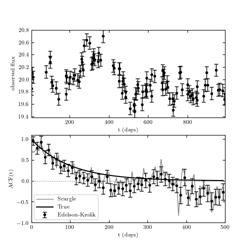
Example of the autocorrelation function for a stochastic process. The top panel shows a simulated light curve generated using a damped random walk model (Section 10.5.4). The bottom panel shows the corresponding autocorrelation function computed using Edelson and Krolik’s DCF method and the Scargle method. The solid line shows the input autocorrelation function used to generate the light curve.

Code output:

Python source code:

# Author: Jake VanderPlas
# License: BSD
#   The figure produced by this code is published in the textbook
#   "Statistics, Data Mining, and Machine Learning in Astronomy" (2013)
#   For more information, see http://astroML.github.com
#   To report a bug or issue, use the following forum:
#    https://groups.google.com/forum/#!forum/astroml-general
import numpy as np
from matplotlib import pyplot as plt

from astroML.time_series import lomb_scargle, generate_damped_RW
from astroML.time_series import ACF_scargle, ACF_EK

#----------------------------------------------------------------------
# This function adjusts matplotlib settings for a uniform feel in the textbook.
# Note that with usetex=True, fonts are rendered with LaTeX.  This may
# result in an error if LaTeX is not installed on your system.  In that case,
# you can set usetex to False.
if "setup_text_plots" not in globals():
    from astroML.plotting import setup_text_plots
setup_text_plots(fontsize=8, usetex=True)

#------------------------------------------------------------
# Generate time-series data:
#  we'll do 1000 days worth of magnitudes

t = np.arange(0, 1E3)
z = 2.0
tau = 300
tau_obs = tau / (1. + z)

np.random.seed(6)
y = generate_damped_RW(t, tau=tau, z=z, xmean=20)

# randomly sample 100 of these
ind = np.arange(len(t))
np.random.shuffle(ind)
ind = ind[:100]
ind.sort()
t = t[ind]
y = y[ind]

# add errors
dy = 0.1
y_obs = np.random.normal(y, dy)

#------------------------------------------------------------
# compute ACF via scargle method
C_S, t_S = ACF_scargle(t, y_obs, dy,
                       n_omega=2. ** 12, omega_max=np.pi / 5.0)

ind = (t_S >= 0) & (t_S <= 500)
t_S = t_S[ind]
C_S = C_S[ind]

#------------------------------------------------------------
# compute ACF via E-K method
C_EK, C_EK_err, bins = ACF_EK(t, y_obs, dy, bins=np.linspace(0, 500, 51))
t_EK = 0.5 * (bins[1:] + bins[:-1])

#------------------------------------------------------------
# Plot the results
fig = plt.figure(figsize=(5, 5))

# plot the input data
ax = fig.add_subplot(211)
ax.errorbar(t, y_obs, dy, fmt='.k', lw=1)
ax.set_xlabel('t (days)')
ax.set_ylabel('observed flux')

# plot the ACF
ax = fig.add_subplot(212)
ax.plot(t_S, C_S, '-', c='gray', lw=1,
        label='Scargle')
ax.errorbar(t_EK, C_EK, C_EK_err, fmt='.k', lw=1,
            label='Edelson-Krolik')
ax.plot(t_S, np.exp(-abs(t_S) / tau_obs), '-k', label='True')
ax.legend(loc=3)

ax.plot(t_S, 0 * t_S, ':', lw=1, c='gray')

ax.set_xlim(0, 500)
ax.set_ylim(-1.0, 1.1)

ax.set_xlabel('t (days)')
ax.set_ylabel('ACF(t)')

plt.show()

[download source: fig_autocorrelation.py]