SDSS Segue Stellar Parameter Pipeline Data

Figure 1.5.

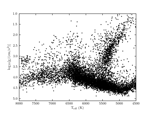
The surface gravity vs. effective temperature plot for the first 10,000 entries from the catalog of stars with SDSS spectra. The rich substructure reflects both stellar physics and the SDSS selection criteria for spectroscopic follow-up. The plume of points centered on Teff ~ 5300 K and log g ~ 3 is dominated by red giant stars, and the locus of points with Teff < 6500 K and log g > 4.5 is dominated by main sequence stars. Stars to the left from the main sequence locus are dominated by the so-called blue horizontal branch stars. The axes are plotted backward for ease of comparison with the classical Hertzsprung-Russell diagram: the luminosity of a star approximately increases upward in this diagram.

Code output:

Python source code:

# Author: Jake VanderPlas
# License: BSD
#   The figure produced by this code is published in the textbook
#   "Statistics, Data Mining, and Machine Learning in Astronomy" (2013)
#   For more information, see http://astroML.github.com
#   To report a bug or issue, use the following forum:
#    https://groups.google.com/forum/#!forum/astroml-general
from matplotlib import pyplot as plt
from astroML.datasets import fetch_sdss_sspp

#----------------------------------------------------------------------
# This function adjusts matplotlib settings for a uniform feel in the textbook.
# Note that with usetex=True, fonts are rendered with LaTeX.  This may
# result in an error if LaTeX is not installed on your system.  In that case,
# you can set usetex to False.
if "setup_text_plots" not in globals():
    from astroML.plotting import setup_text_plots
setup_text_plots(fontsize=8, usetex=True)

#------------------------------------------------------------
# Fetch the data
data = fetch_sdss_sspp()

# select the first 10000 points
data = data[:10000]

# do some reasonable magnitude cuts
rpsf = data['rpsf']
data = data[(rpsf > 15) & (rpsf < 19)]

# get the desired data
logg = data['logg']
Teff = data['Teff']

#------------------------------------------------------------
# Plot the data
fig, ax = plt.subplots(figsize=(5, 3.75))
ax.plot(Teff, logg, marker='.', markersize=2, linestyle='none', color='black')

ax.set_xlim(8000, 4500)
ax.set_ylim(5.1, 1)

ax.set_xlabel(r'$\mathrm{T_{eff}\ (K)}$')
ax.set_ylabel(r'$\mathrm{log_{10}[g / (cm/s^2)]}$')

plt.show()

[download source: fig_SDSS_sspp.py]