Comparison of distributions#
We often ask whether two samples are drawn from the same distribution or, equivalently, whether two sets of measurements imply a difference in the measured quantity. Similarly, we can ask whether a sample is consistent with being drawn from some known distribution.
First, what do we mean by the same distribution? We can describe distributions by their shape, location, and scale. Once we can assume the shape, or likewise once we know from which distribution the sample is drawn (i.e., a Gaussian distribution), the problem simplifies; we now only need to consider two parameters: location and scale.
We can implement different statistical tests depending on the data type (discrete vs. continuous random variables), the assumptions we can make about the underlying distributions and the specific question we ask.
The underlying idea of statistical tests is to use data to compute an appropriate statistic and then compare the resulting data-based value to its expected distribution. As discussed in the preceding section, the expected distribution is evaluated by assuming that the null hypothesis is true. When this expected distribution implies that the data-based value is unlikely to have arisen from it by chance (i.e., a small \(p\) value), the null hypothesis is rejected with some threshold probability \(\alpha\), typically \(0.05\) or \(0.01\) ( \(p < \alpha\)).
Regression toward the mean#
Before proceeding with statistical tests for comparing distributions, we point out a simple statistical selection effect that is sometimes ignored and leads to invalid conclusions.
If two instances of a data set \({x_i}\) are drawn from some distribution, the mean difference between the matched values (i.e., the \(i\)th values from both data sets) will be zero. However, the mean difference can become biased if we use one data set and select a subsample for comparison. For example, if we choose the lowest quartile from the 1st data set, the mean difference between the 2nd and 1st data set will be larger than zero.
This effect is known as regression toward the mean: if a random variable is extreme on its first measurement, it will tend to be closer to the population mean on a second measurement.
Example: In an astronomical context, a commonly related tale states that weather conditions observed at a telescope site today are, typically, not as good as those that would have been inferred from the prior measurements made during the site selection process.
Thus, when selecting a subsample for further study or a control sample for comparison analysis, one has to worry about various statistical selection effects.
Nonparametric methods for comparing distributions#
When the distributions are not known, tests are called nonparametric, or distribution-free tests. The most popular nonparametric test is the Kolmogorov-Smirnov (K-S) test, which compares the cumulative distribution function, \(F(x)\), for two samples, \(\{x1_i\}\), \(i = 1,...,N_1\), and \(\{x2_i\}\), \(i = 1,...,N_2\).
The K-S test is based on the following statistic, which measures the maximum distance of the two cumulative distributions, \(F_1(x1)\) and \(F_2(x2)\),
where \(0 \leq D \leq 1\).
We can visualize \(D\) in the graph below.
import numpy as np
from scipy import stats
import matplotlib.pyplot as plt

np.random.seed(4)
plt.figure(figsize=(12, 8))

plt.step(np.sort(stats.norm.rvs(0,3,25)), np.linspace(0, 1, 25) ,lw = 3)
plt.plot(np.sort(stats.norm.rvs(0,3,1000)), np.linspace(0, 1, 1000), lw=3)

plt.annotate("", xy=(2.3, 0.965), xytext=(2.3, 0.77),
            arrowprops=dict(arrowstyle="<->",lw=2))

plt.text(2.6,0.86, "D", fontsize = 20)

plt.legend(['CDF 1', 'CDF 2'])
plt.title('Comparing CDFs for K-S test')
plt.show()
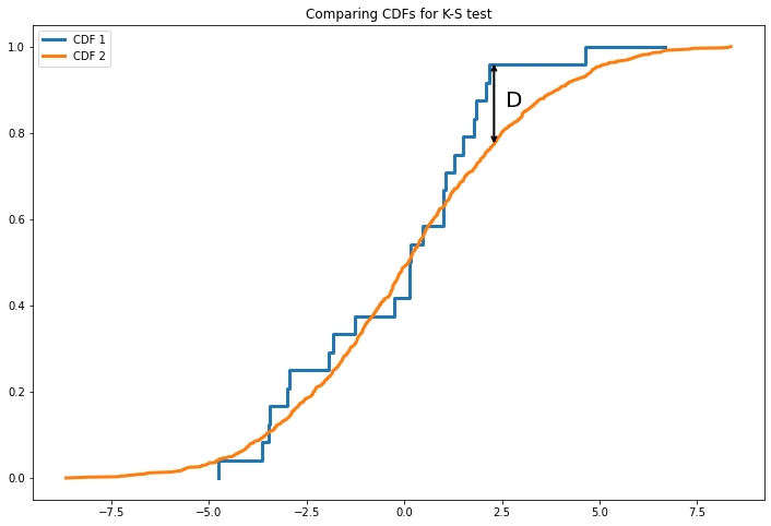
The key question is how often would the value of \(D\) computed from the data arise by chance if the two samples were drawn from the same distribution (the null hypothesis in this case). Surprisingly, this question has a well-defined answer even when we know nothing about the underlying distribution. Kolmogorov showed in 1933 that the probability of obtaining by chance a value of \(D\) larger than the measured value is given by the function
where the argument \(\lambda\) can be accurately described by the following approximation:
where the number of effective data points is computed from
Note that for large \(n_e\), \(\lambda \approx \sqrt{n_e}D\). If the probability that a given value of \(D\) is due to chance is very small (e.g., 0.01 or 0.05), we can reject the null hypothesis that the two samples were drawn from the same underlying distribution.
For \(n_e\) greater than about 10 or so, we can bypass \(\text{eq}\:(1)\) and use the following approximation to evaluate \(D\) corresponding to a given probability \(\alpha\) of obtaining a value at least that large:
$\(D_{KS} = \frac{C(\alpha)}{\sqrt{n_e}} \)$,
where \(C(\alpha = 0.05)= 1.36\) and \(C(\alpha = 0.01)= 1.63\). Note that the ability to reject the null hypothesis (if it really is false) increases with \(\sqrt{n_e}\).
Example: if \(n_e\) = 100, then \(D> D_{KS}\) = 0.163 would arise by chance in only 1% of all trials. If the actual data-based value is indeed 0.163, we can reject the null hypothesis that the data were drawn from the same (unknown) distribution, with our decision being correct 99 out of 100 cases.
We can also use the K-S test to ask, “Is the measured \(f(x)\) consistent with a known reference distribution function \(h(x)\)?” This is known as the “one sample” K-S test, as opposed to the “two sample” K-S test discussed above. In this case, \(N_1 = N\) and \(N_2 = \infty\), and thus \(n_e = N\). Again, a small value of \(Q_{KS}\) (or \(D > D_{KS}\)) indicates that it is unlikely, at the given confidence level set by \(\alpha\), that the data summarized by \(f(x)\) were drawn from \(h(x)\).
The K-S test is sensitive to the underlying distribution’s location, scale, and shape. Additionally, because the test relies on cumulative distributions, it is invariant to the reparametrization of \(x\) (we would get the same answer if we used \(\ln{x}\) instead of \(x\)). The K-S test’s main strength (but also its main weakness) is its ignorance about the underlying distribution. For example, the test is insensitive to details in the differential distribution function (e.g., narrow regions where it drops to zero) and more sensitive near the center distribution than at the tails. The K-S test is not the best choice for distinguishing samples drawn from Gaussian and exponential distributions (see \(\S\)4.7.4).
Python implementation of the K-S test#
The K-S test and its variations can be performed in Python using the routines kstest, ks_2samp, and kstwo from the module scipy.stats.
In the example below, we use np.random.normal to sample a standard Gaussian distribution (\(\mu\) = 0, \(\sigma\) =1). Then we will use kstest, which takes the sample with an underlying distribution we wish to know and compares it against a given distribution. First, we will compare it against a normal distribution and, afterward, a Uniform distribution on [0,1]. We’ll see \(p > 0.05\) when the sample is compared to a normal distribution, whereas \(p < 0.05\) when we compare the sample to a Uniform distribution. Thus, we cannot reject the null hypothesis that the two samples came from the same distribution for the first case, but we can reject it for the second case, which is expected.
import numpy as np
from scipy import stats

np.random.seed(0)
vals = np.random.normal(loc=0, scale=1, size= 1000)

print(f'Normal: {stats.kstest(vals, "norm")}')
print(f'Uniform: {stats.kstest(vals, "uniform")}')
Normal: KstestResult(statistic=0.03737519429804048, pvalue=0.11930823166569182)
Laplace: KstestResult(statistic=0.524, pvalue=3.108930667670788e-256)
Additionally, scipy.stats contains the class ks2_samp, which takes two samples and performs the K-S test. We’ll see again that \(p < 0.05\) when we compare a Uniform distribution to a normal distribution, and thus we can reject the null hypothesis that the two samples came from the same distribution, whereas when we compare two normal distributions, \(p > 0.05\) and we cannot reject the null hypothesis.
import numpy as np
from scipy import stats

np.random.seed(0)
sample1 = np.random.uniform(low=0.0, high=1.0,size=100)
sample2 = np.random.normal(loc=0.0, scale=1.0,size=110)
sample3 = np.random.normal(loc=0.0, scale=1.0,size=95)

print(f'Uniform vs. Normal: {stats.ks_2samp(sample1, sample2)}')
print(f'Normal vs. Normal: {stats.ks_2samp(sample2, sample3)}')
Uniform vs. Normal: KstestResult(statistic=0.4627272727272727, pvalue=1.1459255766510523e-10)
Normal vs. Normal: KstestResult(statistic=0.1645933014354067, pvalue=0.10999225789270017)
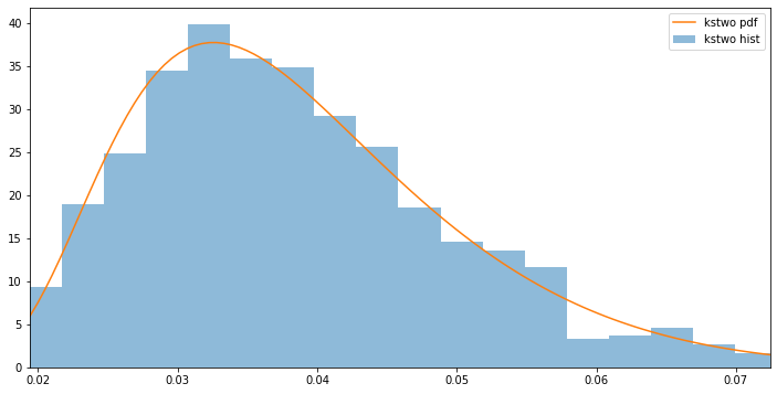
Lastly, we’ll show an example using scipy.stats.kstwo, which performs the two-sided test statistic distribution. Similarly to other scipy.stats classes, we can calculate the first four moments using kstwo.stats. Additionally, we can compare the histogram of random samples generated using kstwo.rvs to the pdf using kstwo.pdf.
import numpy as np
from scipy.stats import kstwo
import matplotlib.pyplot as plt

# Calculate the first four moments for a given n
n = 500
mean, var, skew, kurt = kstwo.stats(n, moments='mvsk')

#Generate random values
r = kstwo.rvs(n, size=1000)

#Plot the ksone pdf and histogram

plt.figure(figsize=(12,6))
x = np.linspace(kstwo.ppf(0.01, n), kstwo.ppf(0.99, n), 100)
plt.hist(r, density=True, bins='auto', histtype='stepfilled', alpha = 0.5, label = 'kstwo hist')
plt.plot(x, kstwo.pdf(x, n),label='kstwo pdf')
plt.xlim([x[0], x[-1]])
plt.legend(loc='best')
plt.show()
The U test and the Wilcoxon test#
The K-S test, as well as other nonparametric methods for comparing distributions, are often sensitive to more than one distribution property, such as the location or scale parameters. We often care about differences in only a particular statistic, such as the mean value, and do not care about the others. For these cases, there exist several nonparametric tests analogous to the better-known classical parametric tests: the \(t\) test and the paired \(t\) test. These are based on the ranks of data points and not their values.
The \(U\) test, or the Mann-Whitney-Wilcoxon test (or the Wilcoxon rank-sum test), is a nonparametric test for testing whether two data sets are drawn from distributions with different location parameters (if the distributions are known to be Gaussian, the standard classical test is called the \(t\) test). The sensitivity of the \(U\) test is dominated by a difference in the medians of the two tested distributions.
The \(U\) statistic is determined using ranks for the full sample obtained by concatenating the two data sets and sorting them while retaining the information about which data set a value came from. To compute the \(U\) statistic, take each value from sample 1 and count the number of observations in sample 2 that have a smaller rank (in the case of identical values, take half a count). The sum of these counts is \(U\), and the minimum of the values with the samples reversed is used to assess the significance. For cases with more than about 20 points per sample, the \(U\) statistic for sample 1 can be more easily computed as
where \(R_1\) is the sum of ranks for sample 1 and analogously for sample 2. The adopted \(U\) statistic is the smaller of the two (note that \(U_1+U_2 = N_1N_2\), which can be used to check computations). The behavior for \(U\) for large samples can be well approximated with a Gaussian distribution, \(\mathcal{N}(\mu_U,\sigma_U)\), of the variable
with
and
A particular case of comparing the means of two data sets is when the data sets have the same size (\(N_1 = N_2 = N\)), and data points are paired. For example, the two data sets could correspond to the same sample measured twice, before and after something that could have affected the values, and we are testing for evidence of a change in means values. The nonparametric Wilcoxon signed-rank test can be used to compare the means of two arbitrary distributions. The test is based on differences \(y_i=x1_i-x2_i\), and the values with \(y_1=0\) are excluded, yielding the new sample size \(m < N\). The sample is ordered by \(|y_i|\), resulting in the rank \(R_i\) for each pair, and each pair is assigned \(\Phi = 1\) if \(x1_i > x2_i\) and 0 otherwise. The Wilcoxon signed-ranked statistic is then
that is, all the ranks with \(y_i > 0\) are summed. Analogously, \(W_{-}\) is the sum of all the ranks with \(y_i < 0\), and the statistic \(T\) is the smaller of the two. For small values of \(m\), the significance of \(T\) can be found in tables. For \(m\) larger than about 20, the behavior of \(T\) can be well approximated with a Gaussian distribution. \(\mathcal{N} (\mu_T, \sigma_T)\), of the variable
with
and
Python implementation of the U test and the Wilcoxon test#
The \(U\) test and Wilcoxon-rank-sum test are implemented in mannwhitneyu and ranksums within the scipy.stats; these are equivalent functions.
import numpy as np
from scipy import stats
np.random.seed(0)

x, y = np.random.normal(0, 1, size=(2, 1000))
print(stats.mannwhitneyu(x, y))
MannwhitneyuResult(statistic=482654.0, pvalue=0.17919398705643008)
import numpy as np
from scipy import stats
np.random.seed(0)

x = np.random.normal(-1, 1, 200)
y = np.random.normal(-0.5, 1.5, 300) # same shape but different location and scale parameters

print(stats.ranksums(x, y))

x = np.random.normal(0, 1, 500)
y = np.random.uniform(-0.5, 0.5, 500) # different shapes, same location

print(stats.ranksums(x, y))
RanksumsResult(statistic=-2.6435517147698615, pvalue=0.008204123191145227)
RanksumsResult(statistic=-2.1280433697217225, pvalue=0.03333348790392057)
Python implementation of Wilcoxon signed-rank test#
The Wilcoxon signed-rank test can be performed with the function scipy.stats.wilcoxon.
import numpy as np
from scipy import stats
np.random.seed(0)

x, y = np.random.normal(0, 1, size=(2, 1000))
print(stats.wilcoxon(x, y))

a = np.random.normal(0, 1, size=500)
b = np.random.uniform(0, 1, size=500)

print(stats.wilcoxon(a, b))
WilcoxonResult(statistic=238373.0, pvalue=0.19357179019702442)
WilcoxonResult(statistic=29627.0, pvalue=1.8119410593156403e-24)
Comparison of two-dimensional distributions#
For multidimensional distribution, the cumulative probability distribution is not well defined in more than one dimension. Thus, there does not exist a direct analog to the K-S test for distributions that are multidimensional. However, we can use a similar method developed by Fasano and Franceschini, which goes as follows:
Assume we have two sets of data points, \(\{x_i^A, y_i^A\}\), \(i = 1,...,N_A\) and \(\{x_i^B, y_i^B\}\), \(i = 1,...,N_B\). Define four quadrants centered on the point \(\{x_j^A, y_j^A\}\).
Compute the number of data points from each data set in each quadrant.
Record the maximum difference among the four quadrants between the fractions for data sets \(A\) and \(B\).
Repeat for all data points \(\{x_j^A, y_j^A\}\) from sample \(A\) to get the overall maximum difference, \(D_A\), and repeat the same process for sample \(B\). The final statistic is then \(D = (D_A+D_B)/2\)
Note that although it isn’t necessarily true that the distribution of \(D\) is independent of the details of the underlying distributions, Fasano and Franceschini showed that its variation is captured well by the coefficient of correlation, \(\rho\). Using simulated samples, they derived the following behavior analogous to the one-dimensional K-S Test:
This value of \(\lambda\) can be used with \(\text{eq}\:(1)\) to compute the significance level of \(D\) when \(n_e >20\).
Is my distribution really Gaussian?#
When asking, “Is the measured \(f(x)\) consistent with a known reference distribution \(h(x)\)?”, a few standard statistical tests can be used when we know or can assume that both \(h(x)\) and \(f(x)\) are Gaussian distributions. We thus need to first reliably prove that our data is, in fact, consistent with being a Gaussian.
Assume we have a data set \(\{x_i\}\); we want to know if we can reject the null hypothesis that \(\{x_i\}\) was drawn from a Gaussian distribution. We aren’t concerned with scale and location parameters at the moment but only whether the shape of the distribution is Gaussian. Common reasons for deviations from a Gaussian are nonzero skewness, nonzero kurtosis, or a complex combination of deviations. Numerous tests are available in statistical literature which have varying sensitivity to different deviations.
Example: The difference between the mean and median for a given data set is sensitive to nonzero skewness but has no sensitivity whatsoever to changes in kurtosis. Therefore, if one is trying to detect a difference between the Gaussian \(\mathcal{N}(\mu = 4, \sigma = 2)\) and the Poisson distribution with \(\mu=4\), the difference between the mean and the median might be a good test (0 vs. 1/6 for large samples), but it will not catch the difference between a Gaussian and an exponential distribution no matter what the size of the sample.
A common feature of most tests is to predict the distribution of their chosen statistic under the assumption that the null hypothesis is true. An added complexity is whether the test uses any parameter estimates derived from data.
The first test we’ll discuss is the Anderson-Darling test, specialized to the case of a Gaussian distribution. The test is based on the statistic
where \(F_i\) is the \(i\)th value of the cumulative distribution function \(z_i\), which is defined as
and assumed to be in ascending order. In this expression, either one or both of \(\mu\) and \(\sigma\) can be known or determined from data \(\{x_i\}\). Depending on which parameters are determined from data, the statistical behavior of \(A^2\) varies. Furthermore, if both \(\mu\) and \(\sigma\) are determined from data, then \(A^2\) needs to be multiplied by \((1+4/N-25/N^2)\). The specialization to a Gaussian distribution enters when predicting the detailed statistical behavior of \(A^2\), and its values for a few common significance levels \((p)\) are listed in Table \(4.1\). The values corresponding to other significance levels as well as the statistical behavior of \(A^2\) in the case of distributions other than Gaussian can be computed with simple numerical simulations.

Python Implementation of the Anderson-Darling test#
The Anderson–Darling test can be performed with the function scipy.stats.anderson. We’ll find that for this random data set, the Anderson-Darling test statistic is 0.877. If we examine the critical values and significance levels, we can see that the statistic exceeds the critical value corresponding with a significance level of 2.5%; thus, we can reject the null hypothesis at a significance level of 2.5%, but we cannot at a significance level of 1%.
import numpy as np
from scipy import stats

rng = np.random.default_rng(4)
x = rng.random(size = 50)
A, crit, sig = stats.anderson(x,"norm")
print(f"""Anderson-Darling Statistic:  {A}
critical values:  {crit}
significance levels:  {sig}""")
Anderson-Darling Statistic:  0.8770622861248185
critical values:  [0.538 0.613 0.736 0.858 1.021]
significance levels:  [15.  10.   5.   2.5  1. ]
The K-S test can also be used to detect a difference between \(f(x)\) and \(\mathcal{N}(\mu,\sigma)\). A difficulty arises if \(\mu\) and \(\sigma\) are determined from the same data set: in this case, the behavior of \(Q_{KS}\) is different from that given by \(\text{eq}\:(1)\) and has only been determined using Monte Carlo simulations.
Another test for detecting non-Gaussianity in \(\{x_i\}\) is the Shapiro-Wilk test. It is implemented in a number of statistical programs and based on both data values \(x_i\) and data ranks \(R_i\):
where constants \(a_i\) encode the expected values of the order statistics for random variables sampled from the standard normal distribution (the test’s null hypothesis). The Shapiro-Wilk test is very sensitive to non-Gaussian tails of the distribution (“outliers”) but not as much to detailed departures from Gaussianity in the distribution’s core.
Python Implementation of the Shapiro–Wilk test#
The Shapiro–Wilk test is implemented in scipy.stats.shapiro. A value of \(W\) close to 1 indicates that the data is indeed Gaussian. Additionally, it still holds that if \(p < 0.05\), we reject the null hypothesis that the distribution came from a Gaussian.
import numpy as np
from scipy import stats
np.random.seed(0)
x = np.random.normal(0, 1, 1000)
y = np.random.uniform(0, 1, 100)
print(stats.shapiro(x))
print(stats.shapiro(y))
ShapiroResult(statistic=0.9985557794570923, pvalue=0.5914123058319092)
ShapiroResult(statistic=0.9477643966674805, pvalue=0.0005927692400291562)
Often the biggest deviation from Gaussianity is due to so-called “catastrophic outliers,” or largely discrepant values many \(\sigma\) away from \(\mu\).
Example: the overwhelming majority of measurements of fluxes of objects in an astronomical image many follow a Gaussian distribution. However, for just a few of them, unrecognized cosmic rays could have had a significant impact on flux extraction.
A simple method to detect the presence of such outliers is to compare the sample standard deviation, \(s\), and \(\sigma_G\), recalling that \(s\) is equal to
and \(\sigma_G\) is equal to
Even when the outlier fraction is tiny, the ratio \(s/\sigma_G\) can become significantly large. When \(N > 100\), for a Gaussian distribution (i.e., for the null hypothesis), this ratio follows a nearly Gaussian distribution with \(\mu \sim 1\) and with \(\sigma \sim 0.92/\sqrt{N}\).
Example: if you measure \(s/\sigma_G = 1.3\) using a sample with \(N=100\), then you can state that the probability of such a large value appearing by chance is less than 1% and reject the null hypothesis that your sample was drawn from a Gaussian distribution.
Another useful result is that the difference of the mean and the median drawn from a Gaussian distribution also follows a nearly Gaussian distribution with \(\mu \sim 0\) and \(\sigma \sim 0.76s/\sqrt{N}\). Therefore, when \(N>100\), we can define two simple statistics based on the measured values of (\(\mu,q_{50},s, \text{and}\:\sigma_G\)) that both measure departures in terms of Gaussian-like “sigma”:
and
$\(Z_2= 1.1\bigg|\frac{s}{\sigma_G}-1\bigg|\sqrt{N}\)$.
Similar results for the statistical behavior of various statistics can be easily derived using Monte Carlo samples.
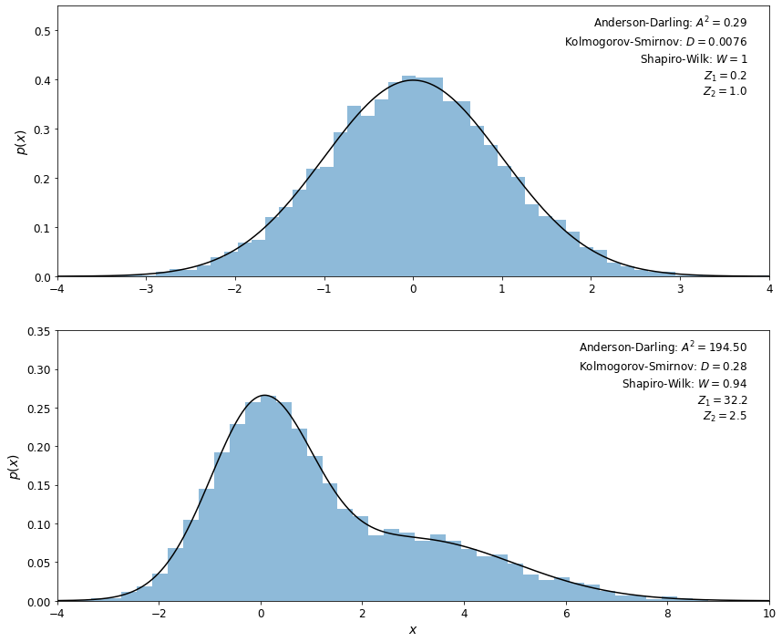
In the example below, we’ll show the results of these tests when applied to samples of \(N = 10,000\) values selected from a Gaussian distribution and from a mixture of two Gaussian distributions. For data that depart from a Gaussian distribution, we expect the Anderson–Darling \(A^2\) statistic to be much larger than 1 (see table 4.1), the K-S \(D\) statistic to be much larger than \(1/\sqrt{N}\), the Shapiro–Wilk \(W\) statistic to be smaller than 1, and \(Z_1\) and \(Z_2\) to be larger than several \(\sigma\). All these tests correctly identify the first data set as being normally distributed, and the second data set as departing from normality.
import numpy as np
from scipy import stats
from matplotlib import pyplot as plt
from astroML.stats import mean_sigma, median_sigmaG

# create distributions
np.random.seed(1)
normal_vals = stats.norm(0, 1).rvs(10000) # singular Gaussian

dual_vals = stats.norm(0, 1).rvs(10000)
dual_vals[:4000] = stats.norm(3,2).rvs(4000) # mixture of two Gaussians

x = np.linspace(-4, 10, 1000)
normal_pdf = stats.norm(0, 1).pdf(x) # pdf for singular Gaussian
dual_pdf = 0.6 * stats.norm(0, 1).pdf(x) + 0.4 * stats.norm(3, 2).pdf(x) #pdf for mixture of two Gaussians

vals = [normal_vals, dual_vals]
pdf = [normal_pdf, dual_pdf]
xlims = [(-4, 4), (-4, 10)]

#------------------------------------------------------------
# Compute the statistics and plot the results
fig = plt.figure(figsize=(14, 12))

for i in range(2):
    ax = fig.add_subplot(2,1,i+1)

    # compute statistics
    A2, sig, crit = stats.anderson(vals[i])
    D, pD = stats.kstest(vals[i], "norm")
    W, pW = stats.shapiro(vals[i])

    mu, sigma = mean_sigma(vals[i], ddof=1)
    median, sigmaG = median_sigmaG(vals[i])

    N = len(vals[i])
    Z1 = 1.3 * abs(mu - median) / sigma * np.sqrt(N)
    Z2 = 1.1 * abs(sigma / sigmaG - 1) * np.sqrt(N)

    # display results in a table
    print(70 * '_')
    print("  Kolmogorov-Smirnov test: D = %.2g  p = %.2g " % (D, pD))
    print("  Anderson-Darling test: A^2 = %.2g" % A2)
    print("    significance  | critical value ")
    print("    --------------|----------------")
    for j in range(len(sig)):
        print("    {0:.2f}          | {1:.1f}%".format(sig[j], crit[j]))
    print("  Shapiro-Wilk test: W = %.2g p = %.2g" % (W, pW))
    print("  Z_1 = %.1f" % Z1)
    print("  Z_2 = %.1f" % Z2)

    # plot a histogram
    ax.hist(vals[i], bins=50, density=True, histtype='stepfilled', alpha=0.5)
    ax.plot(x, pdf[i], '-k')
    ax.set_xlim(xlims[i])

    # print information on the plot
    info = "Anderson-Darling: $A^2 = %.2f$\n" % A2
    info += "Kolmogorov-Smirnov: $D = %.2g$\n" % D
    info += "Shapiro-Wilk: $W = %.2g$\n" % W
    info += "$Z_1 = %.1f$\n$Z_2 = %.1f$" % (Z1, Z2)
    ax.text(0.97, 0.97, info, ha='right', va='top',
            transform=ax.transAxes, fontsize = 12)

    if i == 0:
        ax.set_ylim(0, 0.55)
        ax.tick_params(axis='x', labelsize=12)
        ax.tick_params(axis='y', labelsize=12)
    else:
        ax.set_ylim(0, 0.35)
        ax.set_xlabel('$x$', fontsize = 14)
        ax.tick_params(axis='x', labelsize=12)
        ax.tick_params(axis='y', labelsize=12)

    ax.set_ylabel('$p(x)$', fontsize = 14)

plt.show()
______________________________________________________________________
  Kolmogorov-Smirnov test: D = 0.0076  p = 0.6
  Anderson-Darling test: A^2 = 0.29
    significance  | critical value
    --------------|----------------
    0.58          | 15.0%
    0.66          | 10.0%
    0.79          | 5.0%
    0.92          | 2.5%
    1.09          | 1.0%
  Shapiro-Wilk test: W = 1 p = 0.59
  Z_1 = 0.2
  Z_2 = 1.0
______________________________________________________________________
  Kolmogorov-Smirnov test: D = 0.28  p = 0
  Anderson-Darling test: A^2 = 1.9e+02
    significance  | critical value
    --------------|----------------
    0.58          | 15.0%
    0.66          | 10.0%
    0.79          | 5.0%
    0.92          | 2.5%
    1.09          | 1.0%
  Shapiro-Wilk test: W = 0.94 p = 0
  Z_1 = 32.2
  Z_2 = 2.5
/Library/Frameworks/Python.framework/Versions/3.9/lib/python3.9/site-packages/scipy/stats/morestats.py:1760: UserWarning: p-value may not be accurate for N > 5000.
  warnings.warn("p-value may not be accurate for N > 5000.")
/Library/Frameworks/Python.framework/Versions/3.9/lib/python3.9/site-packages/scipy/stats/morestats.py:1760: UserWarning: p-value may not be accurate for N > 5000.
  warnings.warn("p-value may not be accurate for N > 5000.")
In cases when our empirical distribution fails the tests for Gaussianity, but there is no strong motivation for choosing an alternative specific distribution, a good approach for modeling non-Gaussianity is to adopt the Gram–Charlier series,
where \(z = (x-\mu)/\sigma\) and \(H_k(z)\) are the Hermite polynomials (\(H_0 = 1, H_1 = z, H_2 = z^2-1, H_3 = z^3 - 3z, \text{etc.}\)). For “nearly Gaussian” distributions, even the first few terms of the series provide a good description of \(h(x)\). A related expansion, the Edgeworth series, uses derivatives of \(h(x)\) to derive “correction” factors for a Gaussian distribution.
Is my distribution bimodal?#
It frequently happens in practice that we want to test a hypothesis that the data were drawn from a unimodal distribution (e.g., in the context of studying the bimodal color distribution of galaxies, a bimodal distribution of radio emission from quasars, or the kinematic structure of the Galaxy’s halo). Answering this question can become quite involved, and we discuss it in chapter 5 (see \(\S\)5.7.3).
Parametric methods for comparing distributions#
Given a sample \(\{x_i\}\) that does not fail any test for Gaussianity, one can use a few standard statistical tests for comparing means and variances. They are more efficient than nonparametric tests, but often by much less than a factor of 2. As before, we assume that we are given two samples, \(\{x1_i\}\), which \(i=1,...,N_1\) and \(\{x2_i\}\) with \(i = 1,...,N_2\).
Comparison of Gaussian means using the t test#
If the only question we are asking is whether our data \(\{x1_i\}\) and \(\{x2_i\}\) were drawn from two Gaussian distributions with a different \(\mu\) but the same \(\sigma\), and we were given \(\sigma\), the answer would be simple.
We would first compute the mean values for both samples, \(\overline{x1}\) and \(\overline{x2}\) (where \(\overline{x}\) is equal to \( \overline{x} = \frac{1}{N} \sum ^N_{i=1} x_i \)) and their standard errors, \(\sigma_{\overline{x1}} = \sigma/\sqrt{N_1}\) and analogously for \(\sigma_\overline{x2}\). We would then ask how large is the difference \(\Delta = \overline{x1}-\overline{x2}\) in terms of its expected scatter, \(\sigma_\Delta = \sigma\sqrt{1/N_1^2+1/N_2^2}\): \(M_\sigma = \Delta/ \sigma_\Delta\). The probability that the observed value of \(M\) would arise by chance is given by the Gauss error function as \(p = 1-\text{erf}(M/\sqrt{2})\).
If we do not know \(\sigma\), but need to estimate it from data (with possibly different values for the two sample, \(s_1\) and \(s_2\) (eq \((2)\)), then the ratio \(M_s = \Delta/s_\Delta\), where \(s_\Delta = \sqrt{s_1^2/N_1 + s_2^2/N_2}\), can no longer be described by a Gaussian distribution! Instead, it follows Student’s \(t\) distribution. The number of degrees of freedom depends on whether we assume that the two underlying distributions from which the samples were drawn have the same variances or not. If we can make this assumption, then the relevant statistic (corresponding to \(M_s\)) is
where
is an estimate of the standard error of the difference of the means, and
is an estimator of the common standard deviation of the two samples. The number of degrees of freedom is \(k = (N_1+N_2-2)\). Hence, instead of looking up the significance of \(M_\sigma = \Delta/\sigma_\Delta\) using the Gaussian distribution \(\mathcal{N}(0,1)\), we use the significance corresponding to \(t\) and Student’s \(t\) distribution with \(k\) degrees of freedom. For very large samples, this procedure tends to the simple case with known \(\sigma\) described in the first paragraph because Student’s \(t\) distribution tends to a Gaussian distribution (in other words, \(s\) converges to \(\sigma\)).
A special case of comparing the means of two data sets is when the data sets have the same size \((N_1 =N_2 =N)\)and each pair of data points has the same \(\sigma\) ,but the value of \(\sigma\) is not the same for all pairs (recall the difference between the nonparametric \(U\) and the Wilcoxon tests). In this case, the \(t\) test for paired samples should be used. The expression eq. \((3)\) is still valid, but eq. \((4)\) needs to be modified as
where the covariance between the two samples is
Here the pairs of data points from the two samples need to be properly arranged when summing, and the number of degrees of freedom is \(N-1\).
Python implementation of the \(t\) test#
Variants of the \(t\) test can be computed using the routines ttest_ind and ttest_1samp, available in the module scipy.stats. ttest_ind computes the test for two independent samples; an example of it is shown below.
import numpy as np
from scipy import stats

np.random.seed(0)
rvs1 = stats.norm.rvs(2, 8, 500)
rvs2 = stats.norm.rvs(2, 8, 500) + stats.norm.rvs(0,0.2,500)
print(stats.ttest_ind(rvs1, rvs2))

rvs3 = stats.norm.rvs(6, 8, 500)+ stats.norm.rvs(0,0.2,500)
print(stats.ttest_ind(rvs1, rvs3))
Ttest_indResult(statistic=0.625416390541633, pvalue=0.5318407886123997)
Ttest_indResult(statistic=-8.378738664093502, pvalue=1.8000707268010143e-16)
Additionally,ttest_1samp calculates the T-test for the mean of one group of scores. This is a test for the null hypothesis that the expected mean of a sample of independent observations \(a\) is equal to the given population mean, popmean. Assume we want to check the null hypothesis that the mean of a population is equal to 0.5. We’ll choose a confidence level of 95%
import numpy as np
from scipy import stats

np.random.seed(2)
rvs_1 = stats.uniform.rvs(0,1,size=50)
rvs_2 = stats.norm.rvs(0,1,size=50)

print(stats.ttest_1samp(rvs_1, popmean=0.5))
print(stats.ttest_1samp(rvs_2, popmean=0.5))
Ttest_1sampResult(statistic=-1.3317813022489975, pvalue=0.18909413335928232)
Ttest_1sampResult(statistic=-4.030899743442583, pvalue=0.000193470853688186)
As expected, for the uniform distribution between 0 and 1, we cannot reject the null hypothesis that the mean is 0.5. However, for the normal distribution centered at 0 with a standard deviation of 1 (which has a mean of 0), we can reject the null hypothesis that the population mean is equal to 0.5.
Comparison of Gaussian variances using the F test#
The \(F\) test is used to compare the variances of two samples, \({x1_i}\) and \({x2_i}\), drawn from two unspecified Gaussian distributions. The null hypothesis is that the variances of two samples are equal, and the statistic is based on the ratio of the sample variances. Comparison of Gaussian variances using the \(F\) test
where \(F\) follows Fisher’s \(F\) distribution with \(d_1 = N_1 - 1\) and \(d_2 = N_2 - 1\). Situations when we are interested in only knowing whether \(\sigma_1 < \sigma_2\) or \(\sigma_2 < \sigma_1\) are treated by appropriately using the left and right tails of Fisher’s \(F\) distribution.
Python implementation of the \(F\) test#
Below we will use the \(F\) test to compare the variances of two sample and then print the \(p\) value.
import numpy as np
from scipy import stats

np.random.seed(0)

x, y = np.random.normal(size=(2, 1000))
df1 = len(x) - 1
df2 = len(y) - 1
p = stats.f(df1, df2).cdf(x.var() / y.var())
print(p)
0.7290828317467344