Gausian Mixture Bayes Classification of photometry

Figure 9.6

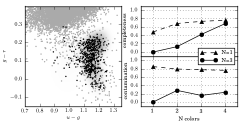
Gaussian mixture Bayes classifier for RR Lyrae stars (see caption of figure 9.3 for details). Here the left panel shows the decision boundary for the three-component model, and the right panel shows the completeness and contamination for both a one-component and three-component mixture model. With all four colors and a three-component model, GMM Bayes achieves a completeness of 0.686 and a contamination of 0.236.

Code output:

@pickle_results: using precomputed results from 'GMMbayes_rrlyrae.pkl'
completeness [[ 0.48175182  0.68613139  0.73722628  0.76642336]
 [ 0.          0.13138686  0.42335766  0.68613139]]
contamination [[ 0.85201794  0.79249448  0.77654867  0.76190476]
 [ 0.          0.28        0.15942029  0.23577236]]

Python source code:

# Author: Jake VanderPlas
# License: BSD
#   The figure produced by this code is published in the textbook
#   "Statistics, Data Mining, and Machine Learning in Astronomy" (2013)
#   For more information, see http://astroML.github.com
#   To report a bug or issue, use the following forum:
#    https://groups.google.com/forum/#!forum/astroml-general
import numpy as np
from matplotlib import pyplot as plt

from astroML.classification import GMMBayes
from astroML.decorators import pickle_results
from astroML.datasets import fetch_rrlyrae_combined
from astroML.utils import split_samples
from astroML.utils import completeness_contamination

#----------------------------------------------------------------------
# This function adjusts matplotlib settings for a uniform feel in the textbook.
# Note that with usetex=True, fonts are rendered with LaTeX.  This may
# result in an error if LaTeX is not installed on your system.  In that case,
# you can set usetex to False.
from astroML.plotting import setup_text_plots
setup_text_plots(fontsize=8, usetex=True)


#----------------------------------------------------------------------
# get data and split into training & testing sets
X, y = fetch_rrlyrae_combined()
X = X[:, [1, 0, 2, 3]]  # rearrange columns for better 1-color results

# GMM-bayes takes several minutes to run, and is order[N^2]
#  truncating the dataset can be useful for experimentation.
#X = X[::10]
#y = y[::10]

(X_train, X_test), (y_train, y_test) = split_samples(X, y, [0.75, 0.25],
                                                     random_state=0)
N_tot = len(y)
N_st = np.sum(y == 0)
N_rr = N_tot - N_st
N_train = len(y_train)
N_test = len(y_test)
N_plot = 5000 + N_rr

#----------------------------------------------------------------------
# perform GMM Bayes
Ncolors = np.arange(1, X.shape[1] + 1)
Ncomp = [1, 3]


@pickle_results('GMMbayes_rrlyrae.pkl')
def compute_GMMbayes(Ncolors, Ncomp):
    classifiers = []
    predictions = []

    for ncm in Ncomp:
        classifiers.append([])
        predictions.append([])
        for nc in Ncolors:
            clf = GMMBayes(ncm, min_covar=1E-5, covariance_type='full')
            clf.fit(X_train[:, :nc], y_train)
            y_pred = clf.predict(X_test[:, :nc])

            classifiers[-1].append(clf)
            predictions[-1].append(y_pred)

    return classifiers, predictions

classifiers, predictions = compute_GMMbayes(Ncolors, Ncomp)

completeness, contamination = completeness_contamination(predictions, y_test)

print "completeness", completeness
print "contamination", contamination

#------------------------------------------------------------
# Compute the decision boundary
clf = classifiers[1][1]
xlim = (0.7, 1.35)
ylim = (-0.15, 0.4)

xx, yy = np.meshgrid(np.linspace(xlim[0], xlim[1], 71),
                     np.linspace(ylim[0], ylim[1], 81))

Z = clf.predict_proba(np.c_[yy.ravel(), xx.ravel()])
Z = Z[:, 1].reshape(xx.shape)

#----------------------------------------------------------------------
# plot the results
fig = plt.figure(figsize=(5, 2.5))
fig.subplots_adjust(bottom=0.15, top=0.95, hspace=0.0,
                    left=0.1, right=0.95, wspace=0.2)

# left plot: data and decision boundary
ax = fig.add_subplot(121)
im = ax.scatter(X[-N_plot:, 1], X[-N_plot:, 0], c=y[-N_plot:],
                s=4, lw=0, cmap=plt.cm.binary, zorder=2)
im.set_clim(-0.5, 1)

im = ax.imshow(Z, origin='lower', aspect='auto',
               cmap=plt.cm.binary, zorder=1,
               extent=xlim + ylim)
im.set_clim(0, 1.5)

ax.contour(xx, yy, Z, [0.5], colors='k')

ax.set_xlim(xlim)
ax.set_ylim(ylim)

ax.set_xlabel('$u-g$')
ax.set_ylabel('$g-r$')

# plot completeness vs Ncolors
ax = fig.add_subplot(222)
ax.plot(Ncolors, completeness[0], '^--k', ms=6, label='N=%i' % Ncomp[0])
ax.plot(Ncolors, completeness[1], 'o-k', ms=6, label='N=%i' % Ncomp[1])

ax.xaxis.set_major_locator(plt.MultipleLocator(1))
ax.yaxis.set_major_locator(plt.MultipleLocator(0.2))
ax.xaxis.set_major_formatter(plt.NullFormatter())

ax.set_ylabel('completeness')
ax.set_xlim(0.5, 4.5)
ax.set_ylim(-0.1, 1.1)
ax.grid(True)

# plot contamination vs Ncolors
ax = fig.add_subplot(224)
ax.plot(Ncolors, contamination[0], '^--k', ms=6, label='N=%i' % Ncomp[0])
ax.plot(Ncolors, contamination[1], 'o-k', ms=6, label='N=%i' % Ncomp[1])
ax.legend(loc='lower right',
          bbox_to_anchor=(1.0, 0.78))

ax.xaxis.set_major_locator(plt.MultipleLocator(1))
ax.yaxis.set_major_locator(plt.MultipleLocator(0.2))
ax.xaxis.set_major_formatter(plt.FormatStrFormatter('%i'))

ax.set_xlabel('N colors')
ax.set_ylabel('contamination')
ax.set_xlim(0.5, 4.5)
ax.set_ylim(-0.1, 1.1)
ax.grid(True)

plt.show()

[download source: fig_rrlyrae_GMMbayes.py]