RR Lyrae ROC Curves

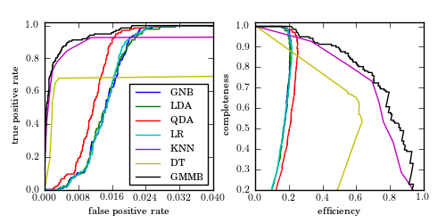
Figure 9.17

ROC curves (left panel) and completeness-efficiency curves (left panel) for the four-color RR Lyrae data using several of the classifiers explored in this chapter: Gaussian naive Bayes (GNB), linear discriminant analysis (LDA), quadratic discriminant analysis (QDA), logistic regression (LR), K -nearest-neighbor classification (KNN), decision tree classification (DT), and GMM Bayes classification (GMMB).

Code output:

GaussianNB
LDA
QDA
LogisticRegression
KNeighborsClassifier
DecisionTreeClassifier
GMMBayes

Python source code:

# Author: Jake VanderPlas
# License: BSD
#   The figure produced by this code is published in the textbook
#   "Statistics, Data Mining, and Machine Learning in Astronomy" (2013)
#   For more information, see http://astroML.github.com
#   To report a bug or issue, use the following forum:
#    https://groups.google.com/forum/#!forum/astroml-general
import numpy as np
from matplotlib import pyplot as plt

from sklearn.naive_bayes import GaussianNB
from sklearn.lda import LDA
from sklearn.qda import QDA
from sklearn.linear_model import LogisticRegression
from sklearn.neighbors import KNeighborsClassifier
from sklearn.tree import DecisionTreeClassifier
from astroML.classification import GMMBayes

from sklearn.metrics import precision_recall_curve, roc_curve

from astroML.utils import split_samples, completeness_contamination
from astroML.datasets import fetch_rrlyrae_combined

#----------------------------------------------------------------------
# This function adjusts matplotlib settings for a uniform feel in the textbook.
# Note that with usetex=True, fonts are rendered with LaTeX.  This may
# result in an error if LaTeX is not installed on your system.  In that case,
# you can set usetex to False.
from astroML.plotting import setup_text_plots
setup_text_plots(fontsize=8, usetex=True)

#----------------------------------------------------------------------
# get data and split into training & testing sets
X, y = fetch_rrlyrae_combined()
y = y.astype(int)
(X_train, X_test), (y_train, y_test) = split_samples(X, y, [0.75, 0.25],
                                                     random_state=0)


#------------------------------------------------------------
# Fit all the models to the training data
def compute_models(*args):
    names = []
    probs = []
    for classifier, kwargs in args:
        print classifier.__name__
        clf = classifier(**kwargs)
        clf.fit(X_train, y_train)
        y_probs = clf.predict_proba(X_test)[:, 1]

        names.append(classifier.__name__)
        probs.append(y_probs)

    return names, probs

names, probs = compute_models((GaussianNB, {}),
                              (LDA, {}),
                              (QDA, {}),
                              (LogisticRegression,
                               dict(class_weight='auto')),
                              (KNeighborsClassifier,
                               dict(n_neighbors=10)),
                              (DecisionTreeClassifier,
                               dict(random_state=0, max_depth=12,
                                    criterion='entropy')),
                              (GMMBayes, dict(n_components=3, min_covar=1E-5,
                                              covariance_type='full')))

#------------------------------------------------------------
# Plot ROC curves and completeness/efficiency
fig = plt.figure(figsize=(5, 2.5))
fig.subplots_adjust(left=0.1, right=0.95, bottom=0.15, top=0.9, wspace=0.25)


# ax2 will show roc curves
ax1 = plt.subplot(121)

# ax1 will show completeness/efficiency
ax2 = plt.subplot(122)

labels = dict(GaussianNB='GNB',
              LDA='LDA',
              QDA='QDA',
              KNeighborsClassifier='KNN',
              DecisionTreeClassifier='DT',
              GMMBayes='GMMB',
              LogisticRegression='LR')

thresholds = np.linspace(0, 1, 1001)[:-1]

# iterate through and show results
for name, y_prob in zip(names, probs):
    fpr, tpr, thresh = roc_curve(y_test, y_prob)

    # add (0, 0) as first point
    fpr = np.concatenate([[0], fpr])
    tpr = np.concatenate([[0], tpr])

    ax1.plot(fpr, tpr, label=labels[name])

    comp = np.zeros_like(thresholds)
    cont = np.zeros_like(thresholds)
    for i, t in enumerate(thresholds):
        y_pred = (y_prob >= t)
        comp[i], cont[i] = completeness_contamination(y_pred, y_test)
    ax2.plot(1 - cont, comp, label=labels[name])

ax1.set_xlim(0, 0.04)
ax1.set_ylim(0, 1.02)
ax1.xaxis.set_major_locator(plt.MaxNLocator(5))
ax1.set_xlabel('false positive rate')
ax1.set_ylabel('true positive rate')
ax1.legend(loc=4)

ax2.set_xlabel('efficiency')
ax2.set_ylabel('completeness')
ax2.set_xlim(0, 1.0)
ax2.set_ylim(0.2, 1.02)

plt.show()

[download source: fig_ROC_curve.py]