Total Least Squares Figure

Figure 8.6

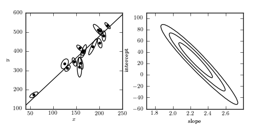
A linear fit to data with correlated errors in x and y. In the literature, this is often referred to as total least squares or errors-in-variables fitting. The left panel shows the lines of best fit; the right panel shows the likelihood contours in slope/intercept space. The points are the same set used for the examples in Hogg, Bovy & Lang 2010.

Code output:

Optimization terminated successfully.
         Current function value: 55.711167
         Iterations: 88
         Function evaluations: 164

Python source code:

# Author: Jake VanderPlas
# License: BSD
#   The figure produced by this code is published in the textbook
#   "Statistics, Data Mining, and Machine Learning in Astronomy" (2013)
#   For more information, see http://astroML.github.com
#   To report a bug or issue, use the following forum:
#    https://groups.google.com/forum/#!forum/astroml-general
import numpy as np
from scipy import optimize
from matplotlib import pyplot as plt
from matplotlib.patches import Ellipse

from astroML.linear_model import TLS_logL
from astroML.plotting.mcmc import convert_to_stdev
from astroML.datasets import fetch_hogg2010test

#----------------------------------------------------------------------
# This function adjusts matplotlib settings for a uniform feel in the textbook.
# Note that with usetex=True, fonts are rendered with LaTeX.  This may
# result in an error if LaTeX is not installed on your system.  In that case,
# you can set usetex to False.
from astroML.plotting import setup_text_plots
setup_text_plots(fontsize=8, usetex=True)


#------------------------------------------------------------
# Define some convenience functions

# translate between typical slope-intercept representation,
# and the normal vector representation
def get_m_b(beta):
    b = np.dot(beta, beta) / beta[1]
    m = -beta[0] / beta[1]
    return m, b


def get_beta(m, b):
    denom = (1 + m * m)
    return np.array([-b * m / denom, b / denom])


# compute the ellipse pricipal axes and rotation from covariance
def get_principal(sigma_x, sigma_y, rho_xy):
    sigma_xy2 = rho_xy * sigma_x * sigma_y

    alpha = 0.5 * np.arctan2(2 * sigma_xy2,
                             (sigma_x ** 2 - sigma_y ** 2))
    tmp1 = 0.5 * (sigma_x ** 2 + sigma_y ** 2)
    tmp2 = np.sqrt(0.25 * (sigma_x ** 2 - sigma_y ** 2) ** 2 + sigma_xy2 ** 2)

    return np.sqrt(tmp1 + tmp2), np.sqrt(tmp1 - tmp2), alpha


# plot ellipses
def plot_ellipses(x, y, sigma_x, sigma_y, rho_xy, factor=2, ax=None):
    if ax is None:
        ax = plt.gca()

    sigma1, sigma2, alpha = get_principal(sigma_x, sigma_y, rho_xy)

    for i in range(len(x)):
        ax.add_patch(Ellipse((x[i], y[i]),
                             factor * sigma1[i], factor * sigma2[i],
                             alpha[i] * 180. / np.pi,
                             fc='none', ec='k'))

#------------------------------------------------------------
# We'll use the data from table 1 of Hogg et al. 2010
data = fetch_hogg2010test()
data = data[5:]  # no outliers
x = data['x']
y = data['y']
sigma_x = data['sigma_x']
sigma_y = data['sigma_y']
rho_xy = data['rho_xy']

#------------------------------------------------------------
# Find best-fit parameters
X = np.vstack((x, y)).T
dX = np.zeros((len(x), 2, 2))
dX[:, 0, 0] = sigma_x ** 2
dX[:, 1, 1] = sigma_y ** 2
dX[:, 0, 1] = dX[:, 1, 0] = rho_xy * sigma_x * sigma_y

min_func = lambda beta: -TLS_logL(beta, X, dX)
beta_fit = optimize.fmin(min_func,
                         x0=[-1, 1])

#------------------------------------------------------------
# Plot the data and fits
fig = plt.figure(figsize=(5, 2.5))
fig.subplots_adjust(left=0.1, right=0.95, wspace=0.25,
                    bottom=0.15, top=0.9)

#------------------------------------------------------------
# first let's visualize the data
ax = fig.add_subplot(121)
ax.scatter(x, y, c='k', s=9)
plot_ellipses(x, y, sigma_x, sigma_y, rho_xy, ax=ax)

#------------------------------------------------------------
# plot the best-fit line
m_fit, b_fit = get_m_b(beta_fit)
x_fit = np.linspace(0, 300, 10)
ax.plot(x_fit, m_fit * x_fit + b_fit, '-k')

ax.set_xlim(40, 250)
ax.set_ylim(100, 600)
ax.set_xlabel('$x$')
ax.set_ylabel('$y$')

#------------------------------------------------------------
# plot the likelihood contour in m, b
ax = fig.add_subplot(122)
m = np.linspace(1.7, 2.8, 100)
b = np.linspace(-60, 110, 100)
logL = np.zeros((len(m), len(b)))

for i in range(len(m)):
    for j in range(len(b)):
        logL[i, j] = TLS_logL(get_beta(m[i], b[j]), X, dX)

ax.contour(m, b, convert_to_stdev(logL.T),
           levels=(0.683, 0.955, 0.997),
           colors='k')
ax.set_xlabel('slope')
ax.set_ylabel('intercept')
ax.set_xlim(1.7, 2.8)
ax.set_ylim(-60, 110)

plt.show()

[download source: fig_total_least_squares.py]