Cosmology Regression Example

Figure 8.2

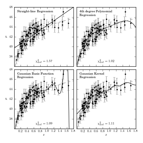
Various regression fits to the distance modulus vs. redshift relation for a simulated set of 100 supernovas, selected from a distribution with . Gaussian basis functions have 15 Gaussians evenly spaced between z = 0 and 2, with widths of 0.14. Kernel regression uses a Gaussian kernel with width 0.1.

Code output:

Python source code:

# Author: Jake VanderPlas
# License: BSD
#   The figure produced by this code is published in the textbook
#   "Statistics, Data Mining, and Machine Learning in Astronomy" (2013)
#   For more information, see http://astroML.github.com
#   To report a bug or issue, use the following forum:
#    https://groups.google.com/forum/#!forum/astroml-general
import numpy as np
from matplotlib import pyplot as plt
from scipy.stats import lognorm

from astroML.cosmology import Cosmology
from astroML.datasets import generate_mu_z
from astroML.linear_model import LinearRegression, PolynomialRegression,\
    BasisFunctionRegression, NadarayaWatson

#----------------------------------------------------------------------
# This function adjusts matplotlib settings for a uniform feel in the textbook.
# Note that with usetex=True, fonts are rendered with LaTeX.  This may
# result in an error if LaTeX is not installed on your system.  In that case,
# you can set usetex to False.
from astroML.plotting import setup_text_plots
setup_text_plots(fontsize=8, usetex=True)

#------------------------------------------------------------
# Generate data
z_sample, mu_sample, dmu = generate_mu_z(100, random_state=0)

cosmo = Cosmology()
z = np.linspace(0.01, 2, 1000)
mu_true = np.asarray(map(cosmo.mu, z))

#------------------------------------------------------------
# Define our classifiers
basis_mu = np.linspace(0, 2, 15)[:, None]
basis_sigma = 3 * (basis_mu[1] - basis_mu[0])

subplots = [221, 222, 223, 224]
classifiers = [LinearRegression(),
               PolynomialRegression(4),
               BasisFunctionRegression('gaussian',
                                       mu=basis_mu, sigma=basis_sigma),
               NadarayaWatson('gaussian', h=0.1)]
text = ['Straight-line Regression',
        '4th degree Polynomial\n Regression',
        'Gaussian Basis Function\n Regression',
        'Gaussian Kernel\n Regression']

# number of constraints of the model.  Because
# Nadaraya-watson is just a weighted mean, it has only one constraint
n_constraints = [2, 5, len(basis_mu) + 1, 1]

#------------------------------------------------------------
# Plot the results
fig = plt.figure(figsize=(5, 5))
fig.subplots_adjust(left=0.1, right=0.95,
                    bottom=0.1, top=0.95,
                    hspace=0.05, wspace=0.05)

for i in range(4):
    ax = fig.add_subplot(subplots[i])

    # fit the data
    clf = classifiers[i]
    clf.fit(z_sample[:, None], mu_sample, dmu)

    mu_sample_fit = clf.predict(z_sample[:, None])
    mu_fit = clf.predict(z[:, None])

    chi2_dof = (np.sum(((mu_sample_fit - mu_sample) / dmu) ** 2)
                / (len(mu_sample) - n_constraints[i]))

    ax.plot(z, mu_fit, '-k')
    ax.plot(z, mu_true, '--', c='gray')
    ax.errorbar(z_sample, mu_sample, dmu, fmt='.k', ecolor='gray', lw=1)

    ax.text(0.5, 0.05, r"$\chi^2_{\rm dof} = %.2f$" % chi2_dof,
            ha='center', va='bottom', transform=ax.transAxes)

    ax.set_xlim(0.01, 1.8)
    ax.set_ylim(36.01, 48)
    ax.text(0.05, 0.95, text[i], ha='left', va='top',
            transform=ax.transAxes)

    if i in (0, 2):
        ax.set_ylabel(r'$\mu$')
    else:
        ax.yaxis.set_major_formatter(plt.NullFormatter())

    if i in (2, 3):
        ax.set_xlabel(r'$z$')
    else:
        ax.xaxis.set_major_formatter(plt.NullFormatter())

plt.show()

[download source: fig_regression_mu_z.py]