PCA Reconstruction of a spectrum

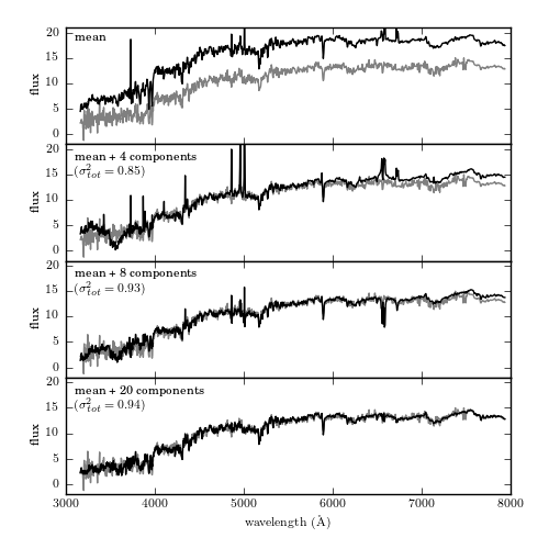
Figure 7.6

The reconstruction of a particular spectrum from its eigenvectors. The input spectrum is shown in gray, and the partial reconstruction for progressively more terms is shown in black. The top panel shows only the mean of the set of spectra. By the time 20 PCA components are added, the reconstruction is very close to the input, as indicated by the expected total variance of 94%.

Code output:

Python source code:

# Author: Jake VanderPlas
# License: BSD
#   The figure produced by this code is published in the textbook
#   "Statistics, Data Mining, and Machine Learning in Astronomy" (2013)
#   For more information, see http://astroML.github.com
#   To report a bug or issue, use the following forum:
#    https://groups.google.com/forum/#!forum/astroml-general
import numpy as np
from matplotlib import pyplot as plt

from sklearn.decomposition import PCA

from astroML.datasets import sdss_corrected_spectra
from astroML.decorators import pickle_results

#----------------------------------------------------------------------
# This function adjusts matplotlib settings for a uniform feel in the textbook.
# Note that with usetex=True, fonts are rendered with LaTeX.  This may
# result in an error if LaTeX is not installed on your system.  In that case,
# you can set usetex to False.
from astroML.plotting import setup_text_plots
setup_text_plots(fontsize=8, usetex=True)


#------------------------------------------------------------
# Download data
data = sdss_corrected_spectra.fetch_sdss_corrected_spectra()
spectra = sdss_corrected_spectra.reconstruct_spectra(data)
wavelengths = sdss_corrected_spectra.compute_wavelengths(data)

#------------------------------------------------------------
# Compute PCA components

# Eigenvalues can be computed using PCA as in the commented code below:

#from sklearn.decomposition import PCA
#pca = PCA()
#pca.fit(spectra)
#evals = pca.explained_variance_ratio_
#evals_cs = evals.cumsum()

#  because the spectra have been reconstructed from masked values, this
#  is not exactly correct in this case: we'll use the values computed
#  in the file compute_sdss_pca.py
evals = data['evals'] ** 2
evals_cs = evals.cumsum()
evals_cs /= evals_cs[-1]
evecs = data['evecs']
spec_mean = spectra.mean(0)

#------------------------------------------------------------
# Find the coefficients of a particular spectrum
spec = spectra[1]
coeff = np.dot(evecs, spec - spec_mean)

#------------------------------------------------------------
# Plot the sequence of reconstructions
fig = plt.figure(figsize=(5, 5))
fig.subplots_adjust(hspace=0, top=0.95, bottom=0.1, left=0.12, right=0.93)

for i, n in enumerate([0, 4, 8, 20]):
    ax = fig.add_subplot(411 + i)
    ax.plot(wavelengths, spec, '-', c='gray')
    ax.plot(wavelengths, spec_mean + np.dot(coeff[:n], evecs[:n]), '-k')

    if i < 3:
        ax.xaxis.set_major_formatter(plt.NullFormatter())

    ax.set_ylim(-2, 21)
    ax.set_ylabel('flux')

    if n == 0:
        text = "mean"
    elif n == 1:
        text = "mean + 1 component\n"
        text += r"$(\sigma^2_{tot} = %.2f)$" % evals_cs[n - 1]
    else:
        text = "mean + %i components\n" % n
        text += r"$(\sigma^2_{tot} = %.2f)$" % evals_cs[n - 1]

    ax.text(0.02, 0.93, text, ha='left', va='top', transform=ax.transAxes)

fig.axes[-1].set_xlabel(r'${\rm wavelength\ (\AA)}$')
plt.show()

[download source: fig_spec_reconstruction.py]