PCA Projection of SDSS Spectra

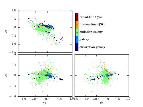
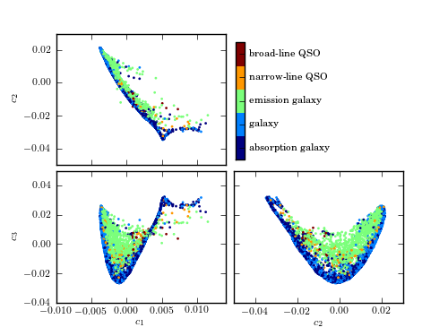
Figure 7.9

A comparison of the classification of quiescent galaxies and sources with strong line emission using LLE and PCA. The top panel shows the segregation of galaxy types as a function of the first three PCA components. The lower panel shows the segregation using the first three LLE dimensions. The preservation of locality in LLE enables nonlinear features within a spectrum (e.g., variation in the width of an emission line) to be captured with fewer components. This results in better segregation of spectral types with fewer dimensions.

Code output:

@pickle_results: using precomputed results from 'spec_LLE.pkl'

Python source code:

# Author: Jake VanderPlas
# License: BSD
#   The figure produced by this code is published in the textbook
#   "Statistics, Data Mining, and Machine Learning in Astronomy" (2013)
#   For more information, see http://astroML.github.com
#   To report a bug or issue, use the following forum:
#    https://groups.google.com/forum/#!forum/astroml-general
import numpy as np
from matplotlib import pyplot as plt
from sklearn import manifold, neighbors

from astroML.datasets import sdss_corrected_spectra
from astroML.datasets import fetch_sdss_corrected_spectra
from astroML.plotting.tools import discretize_cmap
from astroML.decorators import pickle_results

#----------------------------------------------------------------------
# This function adjusts matplotlib settings for a uniform feel in the textbook.
# Note that with usetex=True, fonts are rendered with LaTeX.  This may
# result in an error if LaTeX is not installed on your system.  In that case,
# you can set usetex to False.
from astroML.plotting import setup_text_plots
setup_text_plots(fontsize=8, usetex=True)

#------------------------------------------------------------
# Set up color-map properties
clim = (1.5, 6.5)
cmap = discretize_cmap(plt.cm.jet, 5)
cdict = ['unknown', 'star', 'absorption galaxy',
         'galaxy', 'emission galaxy',
         'narrow-line QSO', 'broad-line QSO']
cticks = [2, 3, 4, 5, 6]
formatter = plt.FuncFormatter(lambda t, *args: cdict[int(np.round(t))])


#------------------------------------------------------------
# Fetch the data; PCA coefficients have been pre-computed
data = fetch_sdss_corrected_spectra()
coeffs_PCA = data['coeffs']
c_PCA = data['lineindex_cln']
spec = sdss_corrected_spectra.reconstruct_spectra(data)
color = data['lineindex_cln']


#------------------------------------------------------------
# Compute the LLE projection; save the results
@pickle_results("spec_LLE.pkl")
def compute_spec_LLE(n_neighbors=10, out_dim=3):
    # Compute the LLE projection
    LLE = manifold.LocallyLinearEmbedding(n_neighbors, out_dim,
                                          method='modified',
                                          eigen_solver='dense')
    Y_LLE = LLE.fit_transform(spec)
    print " - finished LLE projection"

    # remove outliers for the plot
    BT = neighbors.BallTree(Y_LLE)
    dist, ind = BT.query(Y_LLE, n_neighbors)
    dist_to_n = dist[:, -1]
    dist_to_n -= dist_to_n.mean()
    std = np.std(dist_to_n)
    flag = (dist_to_n > 0.25 * std)
    print " - removing %i outliers for plot" % flag.sum()

    return Y_LLE[~flag], color[~flag]

coeffs_LLE, c_LLE = compute_spec_LLE(10, 3)


#----------------------------------------------------------------------
# Plot the results:
for (c, coeffs, xlim) in zip([c_PCA, c_LLE],
                             [coeffs_PCA, coeffs_LLE],
                             [(-1.2, 1.0), (-0.01, 0.014)]):
    fig = plt.figure(figsize=(5, 3.75))
    fig.subplots_adjust(hspace=0.05, wspace=0.05)

    # axes for colorbar
    cax = plt.axes([0.525, 0.525, 0.02, 0.35])

    # Create scatter-plots
    scatter_kwargs = dict(s=4, lw=0, edgecolors='none', c=c, cmap=cmap)

    ax1 = plt.subplot(221)
    im1 = ax1.scatter(coeffs[:, 0], coeffs[:, 1], **scatter_kwargs)
    im1.set_clim(clim)
    ax1.set_ylabel('$c_2$')

    ax2 = plt.subplot(223)
    im2 = ax2.scatter(coeffs[:, 0], coeffs[:, 2], **scatter_kwargs)
    im2.set_clim(clim)
    ax2.set_xlabel('$c_1$')
    ax2.set_ylabel('$c_3$')

    ax3 = plt.subplot(224)
    im3 = ax3.scatter(coeffs[:, 1], coeffs[:, 2], **scatter_kwargs)
    im3.set_clim(clim)
    ax3.set_xlabel('$c_2$')

    fig.colorbar(im3, ax=ax3, cax=cax,
                 ticks=cticks,
                 format=formatter)

    ax1.xaxis.set_major_formatter(plt.NullFormatter())
    ax3.yaxis.set_major_formatter(plt.NullFormatter())

    ax1.set_xlim(xlim)
    ax2.set_xlim(xlim)

    for ax in (ax1, ax2, ax3):
        ax.xaxis.set_major_locator(plt.MaxNLocator(5))
        ax.yaxis.set_major_locator(plt.MaxNLocator(5))

plt.show()

[download source: fig_PCA_LLE.py]