Plot the posterior of mu vs g1 with outliers

Figure 5.17

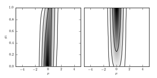
The marginal joint distribution between mu and g_i, as given by eq. 5.100. The left panel shows a point identified as bad (), while the right panel shows a point identified as good().

Code output:

Python source code:

# Author: Jake VanderPlas
# License: BSD
#   The figure produced by this code is published in the textbook
#   "Statistics, Data Mining, and Machine Learning in Astronomy" (2013)
#   For more information, see http://astroML.github.com
#   To report a bug or issue, use the following forum:
#    https://groups.google.com/forum/#!forum/astroml-general
import numpy as np
from matplotlib import pyplot as plt
from scipy.stats import norm
from astroML.plotting.mcmc import convert_to_stdev

#----------------------------------------------------------------------
# This function adjusts matplotlib settings for a uniform feel in the textbook.
# Note that with usetex=True, fonts are rendered with LaTeX.  This may
# result in an error if LaTeX is not installed on your system.  In that case,
# you can set usetex to False.
from astroML.plotting import setup_text_plots
setup_text_plots(fontsize=8, usetex=True)


def p(mu, g1, xi, sigma1, sigma2):
    """Equation 5.97: marginalized likelihood over outliers"""
    L = (g1 * norm.pdf(xi[0], mu, sigma1) +
         (1 - g1) * norm.pdf(xi[0], mu, sigma2))

    mu = mu.reshape(mu.shape + (1,))
    g1 = g1.reshape(g1.shape + (1,))

    return L * np.prod(norm.pdf(xi[1:], mu, sigma1)
                       + norm.pdf(xi[1:], mu, sigma2), -1)

#------------------------------------------------------------
# Sample the points
np.random.seed(138)

N1 = 8
N2 = 2
sigma1 = 1
sigma2 = 3

sigmai = np.zeros(N1 + N2)
sigmai[N2:] = sigma1
sigmai[:N2] = sigma2

xi = np.random.normal(0, sigmai)

#------------------------------------------------------------
# Compute the marginalized posterior for the first and last point
mu = np.linspace(-5, 5, 71)
g1 = np.linspace(0, 1, 11)

L1 = p(mu[:, None], g1, xi, 1, 10)
L1 /= np.max(L1)

L2 = p(mu[:, None], g1, xi[::-1], 1, 10)
L2 /= np.max(L2)

#------------------------------------------------------------
# Plot the results
fig = plt.figure(figsize=(5, 2.5))
fig.subplots_adjust(left=0.1, right=0.95, wspace=0.05,
                    bottom=0.15, top=0.9)

ax1 = fig.add_subplot(121)
ax1.imshow(L1.T, origin='lower', aspect='auto', cmap=plt.cm.binary,
           extent=[mu[0], mu[-1], g1[0], g1[-1]])
ax1.contour(mu, g1, convert_to_stdev(np.log(L1).T),
            levels=(0.683, 0.955, 0.997),
            colors='k')
ax1.set_xlabel(r'$\mu$')
ax1.set_ylabel(r'$g_1$')

ax2 = fig.add_subplot(122)
ax2.imshow(L2.T, origin='lower', aspect='auto', cmap=plt.cm.binary,
           extent=[mu[0], mu[-1], g1[0], g1[-1]])
ax2.contour(mu, g1, convert_to_stdev(np.log(L2).T),
            levels=(0.683, 0.955, 0.997),
            colors='k')
ax2.set_xlabel(r'$\mu$')
ax2.yaxis.set_major_locator(plt.NullLocator())

plt.show()

[download source: fig_outlier_likelihood.py]