Lynden-Bell C- setup

Figure 4.8.

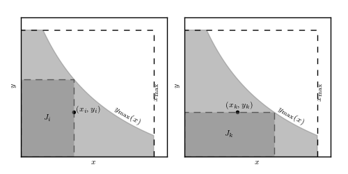
Illustration for the definition of a truncated data set, and for the comparable or associated subset used by the Lynden-Bell C- method. The sample is limited by x < xmax and y < ymax(x) (light-shaded area). Associated sets Ji and Jk are shown by the dark-shaded area.

Code output:

Python source code:

# Author: Jake VanderPlas
# License: BSD
#   The figure produced by this code is published in the textbook
#   "Statistics, Data Mining, and Machine Learning in Astronomy" (2013)
#   For more information, see http://astroML.github.com
#   To report a bug or issue, use the following forum:
#    https://groups.google.com/forum/#!forum/astroml-general
import numpy as np
from matplotlib import pyplot as plt
from matplotlib.patches import Rectangle

#----------------------------------------------------------------------
# This function adjusts matplotlib settings for a uniform feel in the textbook.
# Note that with usetex=True, fonts are rendered with LaTeX.  This may
# result in an error if LaTeX is not installed on your system.  In that case,
# you can set usetex to False.
from astroML.plotting import setup_text_plots
setup_text_plots(fontsize=8, usetex=True)

#------------------------------------------------------------
# Draw the schematic
fig = plt.figure(figsize=(5, 2.5))
fig.subplots_adjust(left=0.06, right=0.95, wspace=0.12)
ax1 = fig.add_subplot(121, xticks=[], yticks=[])
ax2 = fig.add_subplot(122, xticks=[], yticks=[])

# define a convenient function
max_func = lambda t: 1. / (0.5 + t) - 0.5

x = np.linspace(0, 1.0, 100)
ymax = max_func(x)
ymax[ymax > 1] = 1

# draw and label the common background
for ax in (ax1, ax2):
    ax.fill_between(x, 0, ymax, color='gray', alpha=0.5)

    ax.plot([-0.1, 1], [1, 1], '--k', lw=1)

    ax.text(0.7, 0.35, r'$y_{\rm max}(x)$', rotation=-30)

    ax.plot([1, 1], [0, 1], '--k', lw=1)
    ax.text(1.01, 0.5, r'$x_{\rm max}$', ha='left', va='center', rotation=90)

# draw and label J_i in the first axes
xi = 0.4
yi = 0.35
ax1.scatter([xi], [yi], s=16, lw=0, c='k')
ax1.text(xi + 0.02, yi + 0.02, ' $(x_i, y_i)$', ha='left', va='center')
ax1.add_patch(Rectangle((0, 0), xi, max_func(xi), ec='k', fc='gray',
                        linestyle='dashed', lw=1, alpha=0.5))
ax1.text(0.5 * xi, 0.5 * max_func(xi), '$J_i$', ha='center', va='center')

# draw and label J_k in the second axes
ax2.scatter([xi], [yi], s=16, lw=0, c='k')
ax2.text(xi + 0.02, yi + 0.02, ' $(x_k, y_k)$', ha='center', va='bottom')
ax2.add_patch(Rectangle((0, 0), max_func(yi), yi, ec='k', fc='gray',
                        linestyle='dashed', lw=1, alpha=0.5))
ax2.text(0.5 * max_func(yi), 0.5 * yi, '$J_k$', ha='center', va='center')

# adjust the limits of both axes
for ax in (ax1, ax2):
    ax.set_xlim(0, 1.1)
    ax.set_ylim(0, 1.1)
    ax.set_xlabel('$x$')
    ax.set_ylabel('$y$')

plt.show()

[download source: fig_lyndenbell_setup.py]