Bootstrap Calculations of Error on Mean

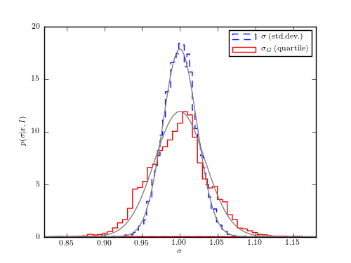
Figure 4.3.

The bootstrap uncertainty estimates for the sample standard deviation (dashed line; see eq. 3.32) and (solid line; see eq. 3.36). The sample consists of N = 1000 values drawn from a Gaussian distribution with and . The bootstrap estimates are based on 10,000 samples. The thin lines show Gaussians with the widths determined as 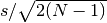(eq. 3.35) for and (eq. 3.37) for .

Code output:

Python source code:

# Author: Jake VanderPlas
# License: BSD
#   The figure produced by this code is published in the textbook
#   "Statistics, Data Mining, and Machine Learning in Astronomy" (2013)
#   For more information, see http://astroML.github.com
#   To report a bug or issue, use the following forum:
#    https://groups.google.com/forum/#!forum/astroml-general
import numpy as np
from scipy.stats import norm
from matplotlib import pyplot as plt

from astroML.resample import bootstrap
from astroML.stats import sigmaG

#----------------------------------------------------------------------
# This function adjusts matplotlib settings for a uniform feel in the textbook.
# Note that with usetex=True, fonts are rendered with LaTeX.  This may
# result in an error if LaTeX is not installed on your system.  In that case,
# you can set usetex to False.
from astroML.plotting import setup_text_plots
setup_text_plots(fontsize=8, usetex=True)

m = 1000  # number of points
n = 10000  # number of bootstraps

#------------------------------------------------------------
# sample values from a normal distribution
np.random.seed(123)
data = norm(0, 1).rvs(m)

#------------------------------------------------------------
# Compute bootstrap resamplings of data
mu1_bootstrap = bootstrap(data, n,  np.std, kwargs=dict(axis=1, ddof=1))
mu2_bootstrap = bootstrap(data, n, sigmaG, kwargs=dict(axis=1))

#------------------------------------------------------------
# Compute the theoretical expectations for the two distributions
x = np.linspace(0.8, 1.2, 1000)

sigma1 = 1. / np.sqrt(2 * (m - 1))
pdf1 = norm(1, sigma1).pdf(x)

sigma2 = 1.06 / np.sqrt(m)
pdf2 = norm(1, sigma2).pdf(x)

#------------------------------------------------------------
# Plot the results
fig, ax = plt.subplots(figsize=(5, 3.75))

ax.hist(mu1_bootstrap, bins=50, normed=True, histtype='step',
        color='blue', ls='dashed', label=r'$\sigma\ {\rm (std. dev.)}$')
ax.plot(x, pdf1, color='gray')

ax.hist(mu2_bootstrap, bins=50, normed=True, histtype='step',
        color='red', label=r'$\sigma_G\ {\rm (quartile)}$')
ax.plot(x, pdf2, color='gray')

ax.set_xlim(0.82, 1.18)

ax.set_xlabel(r'$\sigma$')
ax.set_ylabel(r'$p(\sigma|x,I)$')

ax.legend()

plt.show()

[download source: fig_bootstrap_gaussian.py]