Flux Errors

Figure 3.5.

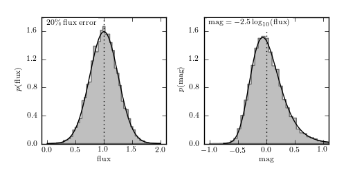
An example of Gaussian flux errors becoming non-Gaussian magnitude errors. The dotted line shows the location of the mean flux; note that this is not coincident with the peak of the magnitude distribution.

Code output:

Python source code:

# Author: Jake VanderPlas
# License: BSD
#   The figure produced by this code is published in the textbook
#   "Statistics, Data Mining, and Machine Learning in Astronomy" (2013)
#   For more information, see http://astroML.github.com
#   To report a bug or issue, use the following forum:
#    https://groups.google.com/forum/#!forum/astroml-general
import numpy as np
from matplotlib import pyplot as plt
from scipy.stats import norm

#----------------------------------------------------------------------
# This function adjusts matplotlib settings for a uniform feel in the textbook.
# Note that with usetex=True, fonts are rendered with LaTeX.  This may
# result in an error if LaTeX is not installed on your system.  In that case,
# you can set usetex to False.
from astroML.plotting import setup_text_plots
setup_text_plots(fontsize=8, usetex=True)

#------------------------------------------------------------
# Create our data

# generate 10000 normally distributed points
np.random.seed(1)
dist = norm(1, 0.25)
flux = dist.rvs(10000)
flux_fit = np.linspace(0.001, 2, 1000)
pdf_flux_fit = dist.pdf(flux_fit)

# transform this distribution into magnitude space
mag = -2.5 * np.log10(flux)
mag_fit = -2.5 * np.log10(flux_fit)
pdf_mag_fit = pdf_flux_fit.copy()
pdf_mag_fit[1:] /= abs(mag_fit[1:] - mag_fit[:-1])
pdf_mag_fit /= np.dot(pdf_mag_fit[1:], abs(mag_fit[1:] - mag_fit[:-1]))

#------------------------------------------------------------
# Plot the result
fig = plt.figure(figsize=(5, 2.5))
fig.subplots_adjust(bottom=0.17, top=0.9,
                    left=0.12, right=0.95, wspace=0.3)

# first plot the flux distribution
ax = fig.add_subplot(121)
ax.hist(flux, bins=np.linspace(0, 2, 50),
        histtype='stepfilled', fc='gray', alpha=0.5, normed=True)
ax.plot(flux_fit, pdf_flux_fit, '-k')
ax.plot([1, 1], [0, 2], ':k', lw=1)
ax.set_xlim(-0.1, 2.1)
ax.set_ylim(0, 1.8)

ax.set_xlabel(r'${\rm flux}$')
ax.set_ylabel(r'$p({\rm flux})$')
ax.yaxis.set_major_locator(plt.MultipleLocator(0.4))
ax.text(0.04, 0.98, r'${\rm 20\%\ flux\ error}$',
        ha='left', va='top', transform=ax.transAxes,
        bbox=dict(ec='none', fc='w'))

# next plot the magnitude distribution
ax = fig.add_subplot(122)
ax.hist(mag, bins=np.linspace(-1, 2, 50),
        histtype='stepfilled', fc='gray', alpha=0.5, normed=True)
ax.plot(mag_fit, pdf_mag_fit, '-k')
ax.plot([0, 0], [0, 2], ':k', lw=1)
ax.set_xlim(-1.1, 1.1)
ax.set_ylim(0, 1.8)
ax.yaxis.set_major_locator(plt.MultipleLocator(0.4))
ax.text(0.04, 0.98, r'${\rm mag} = -2.5\log_{10}({\rm flux})$',
        ha='left', va='top', transform=ax.transAxes,
        bbox=dict(ec='none', fc='w'))

ax.set_xlabel(r'${\rm mag}$')
ax.set_ylabel(r'$p({\rm mag})$')

plt.show()

[download source: fig_flux_errors.py]