Example of central limit theorem

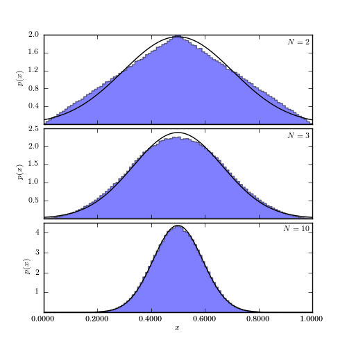
Figure 3.20.

An illustration of the central limit theorem. The histogram in each panel shows the distribution of the mean value of N random variables drawn from the (0, 1) range (a uniform distribution with and W = 1; see eq. 3.39). The distribution for N = 2 has a triangular shape and as N increases it becomes increasingly similar to a Gaussian, in agreement with the central limit theorem. The predicted normal distribution with and is shown by the line. Already for N = 10, the “observed” distribution is essentially the same as the predicted distribution.

Code output:

Python source code:

# Author: Jake VanderPlas
# License: BSD
#   The figure produced by this code is published in the textbook
#   "Statistics, Data Mining, and Machine Learning in Astronomy" (2013)
#   For more information, see http://astroML.github.com
#   To report a bug or issue, use the following forum:
#    https://groups.google.com/forum/#!forum/astroml-general
import numpy as np
from matplotlib import pyplot as plt
from scipy.stats import norm

#----------------------------------------------------------------------
# This function adjusts matplotlib settings for a uniform feel in the textbook.
# Note that with usetex=True, fonts are rendered with LaTeX.  This may
# result in an error if LaTeX is not installed on your system.  In that case,
# you can set usetex to False.
from astroML.plotting import setup_text_plots
setup_text_plots(fontsize=8, usetex=True)

#------------------------------------------------------------
# Generate the uniform samples
N = [2, 3, 10]

np.random.seed(42)
x = np.random.random((max(N), 1E6))

#------------------------------------------------------------
# Plot the results
fig = plt.figure(figsize=(5, 5))
fig.subplots_adjust(hspace=0.05)

for i in range(len(N)):
    ax = fig.add_subplot(3, 1, i + 1)

    # take the mean of the first N[i] samples
    x_i = x[:N[i], :].mean(0)

    # histogram the data
    ax.hist(x_i, bins=np.linspace(0, 1, 101),
            histtype='stepfilled', alpha=0.5, normed=True)

    # plot the expected gaussian pdf
    mu = 0.5
    sigma = 1. / np.sqrt(12 * N[i])
    dist = norm(mu, sigma)
    x_pdf = np.linspace(-0.5, 1.5, 1000)
    ax.plot(x_pdf, dist.pdf(x_pdf), '-k')

    ax.set_xlim(0.0, 1.0)
    ax.set_ylim(0.001, None)

    ax.xaxis.set_major_locator(plt.MultipleLocator(0.2))
    ax.yaxis.set_major_locator(plt.MaxNLocator(5))

    ax.text(0.99, 0.95, r"$N = %i$" % N[i],
            ha='right', va='top', transform=ax.transAxes)

    if i == len(N) - 1:
        ax.xaxis.set_major_formatter(plt.FormatStrFormatter('%.4f'))
        ax.set_xlabel(r'$x$')
    else:
        ax.xaxis.set_major_formatter(plt.NullFormatter())

    ax.set_ylabel('$p(x)$')

plt.show()

[download source: fig_central_limit.py]