Wiener Filter Example

Figure 10.10

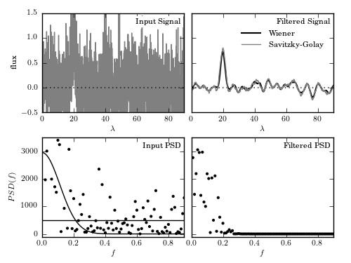
An example of data filtering using a Wiener filter. The upper-left panel shows noisy input data (200 evenly spaced points) with a narrow Gaussian peak centered at x = 20. The bottom panels show the input (left) and Wiener-filtered (right) power spectral density (PSD) distributions. The two curves in the bottom-left panel represent two-component fit to PSD given by eq. 10.20. The upper-right panel shows the result of the Wiener filtering on the input: the Gaussian peak is clearly seen. For comparison, we also plot the result of a fourth-order Savitzky-Golay filter with a window size of lambda = 10.

Code output:

Optimization terminated successfully.
         Current function value: 574032608.556377
         Iterations: 93
         Function evaluations: 180

Python source code:

# Author: Jake VanderPlas
# License: BSD
#   The figure produced by this code is published in the textbook
#   "Statistics, Data Mining, and Machine Learning in Astronomy" (2013)
#   For more information, see http://astroML.github.com
#   To report a bug or issue, use the following forum:
#    https://groups.google.com/forum/#!forum/astroml-general
import numpy as np
from matplotlib import pyplot as plt

from scipy import optimize, fftpack
from astroML.filters import savitzky_golay, wiener_filter

#----------------------------------------------------------------------
# This function adjusts matplotlib settings for a uniform feel in the textbook.
# Note that with usetex=True, fonts are rendered with LaTeX.  This may
# result in an error if LaTeX is not installed on your system.  In that case,
# you can set usetex to False.
from astroML.plotting import setup_text_plots
setup_text_plots(fontsize=8, usetex=True)

#------------------------------------------------------------
# Create the noisy data
np.random.seed(5)
N = 2000
dt = 0.05

t = dt * np.arange(N)
h = np.exp(-0.5 * ((t - 20.) / 1.0) ** 2)
hN = h + np.random.normal(0, 0.5, size=h.shape)

Df = 1. / N / dt
f = fftpack.ifftshift(Df * (np.arange(N) - N / 2))
HN = fftpack.fft(hN)

#------------------------------------------------------------
# Set up the Wiener filter:
#  fit a model to the PSD consisting of the sum of a
#  gaussian and white noise
h_smooth, PSD, P_S, P_N, Phi = wiener_filter(t, hN, return_PSDs=True)

#------------------------------------------------------------
# Use the Savitzky-Golay filter to filter the values
h_sg = savitzky_golay(hN, window_size=201, order=4, use_fft=False)

#------------------------------------------------------------
# Plot the results
N = len(t)
Df = 1. / N / (t[1] - t[0])
f = fftpack.ifftshift(Df * (np.arange(N) - N / 2))
HN = fftpack.fft(hN)

fig = plt.figure(figsize=(5, 3.75))
fig.subplots_adjust(wspace=0.05, hspace=0.25,
                    bottom=0.1, top=0.95,
                    left=0.12, right=0.95)

# First plot: noisy signal
ax = fig.add_subplot(221)
ax.plot(t, hN, '-', c='gray')
ax.plot(t, np.zeros_like(t), ':k')
ax.text(0.98, 0.95, "Input Signal", ha='right', va='top',
        transform=ax.transAxes, bbox=dict(fc='w', ec='none'))

ax.set_xlim(0, 90)
ax.set_ylim(-0.5, 1.5)

ax.xaxis.set_major_locator(plt.MultipleLocator(20))
ax.set_xlabel(r'$\lambda$')
ax.set_ylabel('flux')

# Second plot: filtered signal
ax = plt.subplot(222)
ax.plot(t, np.zeros_like(t), ':k', lw=1)
ax.plot(t, h_smooth, '-k', lw=1.5, label='Wiener')
ax.plot(t, h_sg, '-', c='gray', lw=1, label='Savitzky-Golay')

ax.text(0.98, 0.95, "Filtered Signal", ha='right', va='top',
        transform=ax.transAxes)
ax.legend(loc='upper right', bbox_to_anchor=(0.98, 0.9), frameon=False)

ax.set_xlim(0, 90)
ax.set_ylim(-0.5, 1.5)

ax.yaxis.set_major_formatter(plt.NullFormatter())
ax.xaxis.set_major_locator(plt.MultipleLocator(20))
ax.set_xlabel(r'$\lambda$')

# Third plot: Input PSD
ax = fig.add_subplot(223)
ax.scatter(f[:N / 2], PSD[:N / 2], s=9, c='k', lw=0)
ax.plot(f[:N / 2], P_S[:N / 2], '-k')
ax.plot(f[:N / 2], P_N[:N / 2], '-k')

ax.text(0.98, 0.95, "Input PSD", ha='right', va='top',
        transform=ax.transAxes)

ax.set_ylim(-100, 3500)
ax.set_xlim(0, 0.9)

ax.yaxis.set_major_locator(plt.MultipleLocator(1000))
ax.xaxis.set_major_locator(plt.MultipleLocator(0.2))
ax.set_xlabel('$f$')
ax.set_ylabel('$PSD(f)$')

# Fourth plot: Filtered PSD
ax = fig.add_subplot(224)
filtered_PSD = (Phi * abs(HN)) ** 2
ax.scatter(f[:N / 2], filtered_PSD[:N / 2], s=9, c='k', lw=0)

ax.text(0.98, 0.95, "Filtered PSD", ha='right', va='top',
        transform=ax.transAxes)

ax.set_ylim(-100, 3500)
ax.set_xlim(0, 0.9)

ax.yaxis.set_major_locator(plt.MultipleLocator(1000))
ax.yaxis.set_major_formatter(plt.NullFormatter())
ax.xaxis.set_major_locator(plt.MultipleLocator(0.2))
ax.set_xlabel('$f$')

plt.show()

[download source: fig_wiener_filter.py]