Generalized vs Standard Lomb-Scargle

Figure 10.16

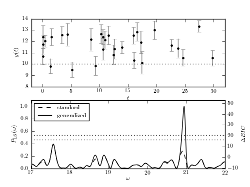
A comparison of the standard and generalized Lomb-Scargle periodograms for a signal y(t) = 10 + sin(2pi t/P) with P = 0.3, corresponding to omega_0 ~ 21. This example is, in some sense, a worst-case scenario for the standard Lomb-Scargle algorithm because there are no sampled points during the times when ytrue < 10, which leads to a gross overestimation of the mean. The bottom panel shows the Lomb-Scargle and generalized Lomb-Scargle periodograms for these data; the generalized method recovers the expected peak as the highest peak, while the standard method incorrectly chooses the peak at omega ~ 17.6 (because it is higher than the true peak at omega_0 ~ 21). The dotted lines show the 1% and 5% significance levels for the highest peak in the generalized periodogram, determined by 1000 bootstrap resamplings (see Section 10.3.2).

Note: This Plot Contains an Error

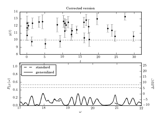
After the book was in press, a reader pointed out that this plot contains a typo. Instead of passing the noisy data to the Lomb-Scargle routine, we had passed the underlying, non-noisy data. This caused an over-estimate of the Lomb-Scargle power.

Because of this, we add two extra plots to this script: the first reproduces the current plot without the typo. In it, we see that for the noisy data, the period is not detected for just ~30 points within ten periods.

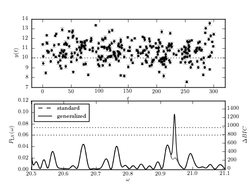
In the second additional plot, we increase the baseline and the number of points by a factor of ten. With this configuration, the peak is detected, and the qualitative aspects of the above discussion hold true.

We regret the error!

Code output:

Python source code:

# Author: Jake VanderPlas
# License: BSD
#   The figure produced by this code is published in the textbook
#   "Statistics, Data Mining, and Machine Learning in Astronomy" (2013)
#   For more information, see http://astroML.github.com
#   To report a bug or issue, use the following forum:
#    https://groups.google.com/forum/#!forum/astroml-general
import numpy as np
from matplotlib import pyplot as plt

from astroML.time_series import \
    lomb_scargle, lomb_scargle_BIC, lomb_scargle_bootstrap

#----------------------------------------------------------------------
# This function adjusts matplotlib settings for a uniform feel in the textbook.
# Note that with usetex=True, fonts are rendered with LaTeX.  This may
# result in an error if LaTeX is not installed on your system.  In that case,
# you can set usetex to False.
from astroML.plotting import setup_text_plots
setup_text_plots(fontsize=8, usetex=True)

#------------------------------------------------------------
# Generate data where y is positive
np.random.seed(0)
N = 30
P = 0.3

t = P / 2 * np.random.random(N) + P * np.random.randint(100, size=N)
y = 10 + np.sin(2 * np.pi * t / P)
dy = 0.5 + 0.5 * np.random.random(N)
y_obs = y + np.random.normal(dy)

omega_0 = 2 * np.pi / P

#######################################################################
# Generate the plot with and without the original typo

for typo in [True, False]:
    #------------------------------------------------------------
    # Compute the Lomb-Scargle Periodogram
    sig = np.array([0.1, 0.01, 0.001])
    omega = np.linspace(17, 22, 1000)

    # Notice the typo: we used y rather than y_obs
    if typo is True:
        P_S = lomb_scargle(t, y, dy, omega, generalized=False)
        P_G = lomb_scargle(t, y, dy, omega, generalized=True)
    else:
        P_S = lomb_scargle(t, y_obs, dy, omega, generalized=False)
        P_G = lomb_scargle(t, y_obs, dy, omega, generalized=True)

    #------------------------------------------------------------
    # Get significance via bootstrap
    D = lomb_scargle_bootstrap(t, y_obs, dy, omega, generalized=True,
                               N_bootstraps=1000, random_state=0)
    sig1, sig5 = np.percentile(D, [99, 95])

    #------------------------------------------------------------
    # Plot the results
    fig = plt.figure(figsize=(5, 3.75))

    # First panel: input data
    ax = fig.add_subplot(211)
    ax.errorbar(t, y_obs, dy, fmt='.k', lw=1, ecolor='gray')
    ax.plot([-2, 32], [10, 10], ':k', lw=1)

    ax.set_xlim(-2, 32)
    ax.set_xlabel('$t$')
    ax.set_ylabel('$y(t)$')

    if typo is False:
        ax.set_title('Corrected version')

    # Second panel: periodogram
    ax = fig.add_subplot(212)
    ax.plot(omega, P_S, '--k', lw=1, label='standard')
    ax.plot(omega, P_G, '-k', lw=1, label='generalized')
    ax.legend(loc=2)

    # plot the significance lines.
    xlim = (omega[0], omega[-1])
    ax.plot(xlim, [sig1, sig1], ':', c='black')
    ax.plot(xlim, [sig5, sig5], ':', c='black')

    # label BIC on the right side
    ax2 = ax.twinx()
    ax2.set_ylim(tuple(lomb_scargle_BIC(ax.get_ylim(), y_obs, dy)))
    ax2.set_ylabel(r'$\Delta BIC$')

    ax.set_xlabel('$\omega$')
    ax.set_ylabel(r'$P_{\rm LS}(\omega)$')
    ax.set_ylim(0, 1.1)


#######################################################################
# Redo the plot without the typo
# We need a larger data range to actually get significant power
# with actual noisy data

#------------------------------------------------------------
# Generate data where y is positive
np.random.seed(0)
N = 300
P = 0.3

t = P / 2 * np.random.random(N) + P * np.random.randint(1000, size=N)
y = 10 + np.sin(2 * np.pi * t / P)
dy = 0.1 + 0.1 * np.random.random(N)
y_obs = y + np.random.normal(dy)

omega_0 = 2 * np.pi / P


#------------------------------------------------------------
# Compute the Lomb-Scargle Periodogram
sig = np.array([0.1, 0.01, 0.001])
omega = np.linspace(20.5, 21.1, 1000)

P_S = lomb_scargle(t, y_obs, dy, omega, generalized=False)
P_G = lomb_scargle(t, y_obs, dy, omega, generalized=True)

#------------------------------------------------------------
# Get significance via bootstrap
D = lomb_scargle_bootstrap(t, y_obs, dy, omega, generalized=True,
                           N_bootstraps=1000, random_state=0)
sig1, sig5 = np.percentile(D, [99, 95])

#------------------------------------------------------------
# Plot the results
fig = plt.figure(figsize=(5, 3.75))

# First panel: input data
ax = fig.add_subplot(211)
ax.errorbar(t, y_obs, dy, fmt='.k', lw=1, ecolor='gray')
ax.plot([-20, 320], [10, 10], ':k', lw=1)

ax.set_xlim(-20, 320)
ax.set_xlabel('$t$')
ax.set_ylabel('$y(t)$')

# Second panel: periodogram
ax = fig.add_subplot(212)
ax.plot(omega, P_S, '--k', lw=1, label='standard')
ax.plot(omega, P_S, '-', c='gray', lw=1)
ax.plot(omega, P_G, '-k', lw=1, label='generalized')
ax.legend(loc=2)

# plot the significance lines.
xlim = (omega[0], omega[-1])
ax.plot(xlim, [sig1, sig1], ':', c='black')
ax.plot(xlim, [sig5, sig5], ':', c='black')

# label BIC on the right side
ax2 = ax.twinx()
ax2.set_ylim(tuple(lomb_scargle_BIC(ax.get_ylim(), y_obs, dy)))
ax2.set_ylabel(r'$\Delta BIC$')

ax.set_xlabel('$\omega$')
ax.set_ylabel(r'$P_{\rm LS}(\omega)$')
ax.set_xlim(xlim)
ax.set_ylim(0, 0.12)

plt.show()

[download source: fig_LS_sg_comparison.py]