BIC for LINEAR light curve

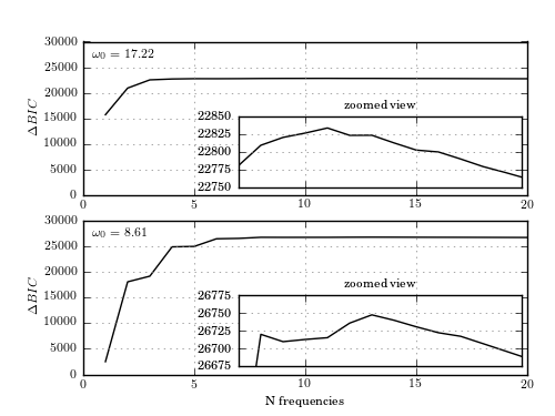
Figure 10.19

BIC as a function of the number of frequency components for the light curve shown in figure 10.18. BIC for the two prominent frequency peaks is shown. The inset panel details the area near the maximum. For both frequencies, the BIC peaks at between 10 and 15 terms; note that a high value of BIC is achieved already with 6 components. Comparing the two, the longer period model (bottom panel) is much more significant.

Code output:

Python source code:

# Author: Jake VanderPlas
# License: BSD
#   The figure produced by this code is published in the textbook
#   "Statistics, Data Mining, and Machine Learning in Astronomy" (2013)
#   For more information, see http://astroML.github.com
#   To report a bug or issue, use the following forum:
#    https://groups.google.com/forum/#!forum/astroml-general
import numpy as np
from matplotlib import pyplot as plt

from astroML.time_series import multiterm_periodogram, lomb_scargle_BIC
from astroML.datasets import fetch_LINEAR_sample

#----------------------------------------------------------------------
# This function adjusts matplotlib settings for a uniform feel in the textbook.
# Note that with usetex=True, fonts are rendered with LaTeX.  This may
# result in an error if LaTeX is not installed on your system.  In that case,
# you can set usetex to False.
from astroML.plotting import setup_text_plots
setup_text_plots(fontsize=8, usetex=True)

#------------------------------------------------------------
# Fetch the data
data = fetch_LINEAR_sample()

t, y, dy = data[14752041].T
omega0 = 17.217

# focus only on the region with the peak
omega1 = np.linspace(17.213, 17.220, 100)
omega2 = 0.5 * omega1

#------------------------------------------------------------
# Compute the delta BIC
terms = np.arange(1, 21)
BIC_max = np.zeros((2, len(terms)))

for i, omega in enumerate([omega1, omega2]):
    for j in range(len(terms)):
        P = multiterm_periodogram(t, y, dy, omega, terms[j])
        BIC = lomb_scargle_BIC(P, y, dy, n_harmonics=terms[j])
        BIC_max[i, j] = BIC.max()

#----------------------------------------------------------------------
# Plot the results
fig = plt.figure(figsize=(5, 3.75))

ax = [fig.add_axes((0.15, 0.53, 0.8, 0.37)),
      fig.add_axes((0.15, 0.1, 0.8, 0.37))]
ax_inset = [fig.add_axes((0.15 + 7 * 0.04, 0.55, 0.79 - 7 * 0.04, 0.17)),
            fig.add_axes((0.15 + 7 * 0.04, 0.12, 0.79 - 7 * 0.04, 0.17))]
ylims = [(22750, 22850),
         (26675, 26775)]
omega0 = [17.22, 8.61]

for i in range(2):
    # Plot full panel
    ax[i].plot(terms, BIC_max[i], '-k')
    ax[i].set_xlim(0, 20)
    ax[i].set_ylim(0, 30000)
    ax[i].text(0.02, 0.95, r"$\omega_0 = %.2f$" % omega0[i],
               ha='left', va='top', transform=ax[i].transAxes)

    ax[i].set_ylabel(r'$\Delta BIC$')
    if i == 1:
        ax[i].set_xlabel('N frequencies')
    ax[i].grid(color='gray')

    # plot inset
    ax_inset[i].plot(terms, BIC_max[i], '-k')
    ax_inset[i].xaxis.set_major_locator(plt.MultipleLocator(5))
    ax_inset[i].xaxis.set_major_formatter(plt.NullFormatter())
    ax_inset[i].yaxis.set_major_locator(plt.MultipleLocator(25))
    ax_inset[i].yaxis.set_major_formatter(plt.FormatStrFormatter('%i'))
    ax_inset[i].set_xlim(7, 19.75)
    ax_inset[i].set_ylim(ylims[i])
    ax_inset[i].set_title('zoomed view')
    ax_inset[i].grid(color='gray')

plt.show()

[download source: fig_LINEAR_BIC.py]