SVM Classification of photometry

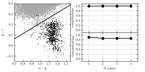
Figure 9.10

SVM applied to the RR Lyrae data (see caption of figure 9.3 for details). With all four colors, SVM achieves a completeness of 1.0 and a contamination of 0.854.

Code output:

@pickle_results: computing results and saving to 'SVM_rrlyrae.pkl'
completeness [0.99270073 1.         1.         1.        ]
contamination [0.90014684 0.85347594 0.85347594 0.85471898]

Python source code:

# Author: Jake VanderPlas
# License: BSD
#   The figure produced by this code is published in the textbook
#   "Statistics, Data Mining, and Machine Learning in Astronomy" (2013)
#   For more information, see http://astroML.github.com
#   To report a bug or issue, use the following forum:
#    https://groups.google.com/forum/#!forum/astroml-general

from __future__ import print_function

import numpy as np
from matplotlib import pyplot as plt

from sklearn.svm import SVC
from astroML.utils.decorators import pickle_results
from astroML.datasets import fetch_rrlyrae_combined
from astroML.utils import split_samples
from astroML.utils import completeness_contamination

#----------------------------------------------------------------------
# This function adjusts matplotlib settings for a uniform feel in the textbook.
# Note that with usetex=True, fonts are rendered with LaTeX.  This may
# result in an error if LaTeX is not installed on your system.  In that case,
# you can set usetex to False.
if "setup_text_plots" not in globals():
    from astroML.plotting import setup_text_plots
setup_text_plots(fontsize=8, usetex=True)

#----------------------------------------------------------------------
# get data and split into training & testing sets
X, y = fetch_rrlyrae_combined()
X = X[:, [1, 0, 2, 3]]  # rearrange columns for better 1-color results

# SVM takes several minutes to run, and is order[N^2]
#  truncating the dataset can be useful for experimentation.
#X = X[::5]
#y = y[::5]

(X_train, X_test), (y_train, y_test) = split_samples(X, y, [0.75, 0.25],
                                                     random_state=0)

N_tot = len(y)
N_st = np.sum(y == 0)
N_rr = N_tot - N_st
N_train = len(y_train)
N_test = len(y_test)
N_plot = 5000 + N_rr

#----------------------------------------------------------------------
# Fit SVM
Ncolors = np.arange(1, X.shape[1] + 1)


@pickle_results('SVM_rrlyrae.pkl')
def compute_SVM(Ncolors):
    classifiers = []
    predictions = []

    for nc in Ncolors:
        # perform support vector classification
        clf = SVC(kernel='linear', class_weight='balanced')
        clf.fit(X_train[:, :nc], y_train)
        y_pred = clf.predict(X_test[:, :nc])

        classifiers.append(clf)
        predictions.append(y_pred)

    return classifiers, predictions

classifiers, predictions = compute_SVM(Ncolors)

completeness, contamination = completeness_contamination(predictions, y_test)

print("completeness", completeness)
print("contamination", contamination)

#------------------------------------------------------------
# compute the decision boundary
clf = classifiers[1]
w = clf.coef_[0]
a = -w[0] / w[1]
yy = np.linspace(-0.1, 0.4)
xx = a * yy - clf.intercept_[0] / w[1]

#----------------------------------------------------------------------
# plot the results
fig = plt.figure(figsize=(5, 2.5))
fig.subplots_adjust(bottom=0.15, top=0.95, hspace=0.0,
                    left=0.1, right=0.95, wspace=0.2)

# left plot: data and decision boundary
ax = fig.add_subplot(121)
ax.plot(xx, yy, '-k')
im = ax.scatter(X[-N_plot:, 1], X[-N_plot:, 0], c=y[-N_plot:],
                s=4, lw=0, cmap=plt.cm.binary, zorder=2)
im.set_clim(-0.5, 1)

ax.set_xlim(0.7, 1.35)
ax.set_ylim(-0.15, 0.4)

ax.set_xlabel('$u-g$')
ax.set_ylabel('$g-r$')

# plot completeness vs Ncolors
ax = fig.add_subplot(222)
ax.plot(Ncolors, completeness, 'o-k', ms=6)

ax.xaxis.set_major_locator(plt.MultipleLocator(1))
ax.yaxis.set_major_locator(plt.MultipleLocator(0.2))
ax.xaxis.set_major_formatter(plt.NullFormatter())

ax.set_ylabel('completeness')
ax.set_xlim(0.5, 4.5)
ax.set_ylim(-0.1, 1.1)
ax.grid(True)

# plot contamination vs Ncolors
ax = fig.add_subplot(224)
ax.plot(Ncolors, contamination, 'o-k', ms=6)

ax.xaxis.set_major_locator(plt.MultipleLocator(1))
ax.yaxis.set_major_locator(plt.MultipleLocator(0.2))
ax.xaxis.set_major_formatter(plt.FormatStrFormatter('%i'))

ax.set_xlabel('N colors')
ax.set_ylabel('contamination')
ax.set_xlim(0.5, 4.5)
ax.set_ylim(-0.1, 1.1)
ax.grid(True)

plt.show()

[download source: fig_rrlyrae_svm.py]