Perform Outlier Rejection with MCMC
Figure 8.9
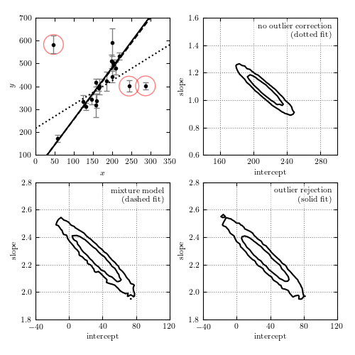
Bayesian outlier detection for the same data as shown in figure 8.8. The top-left panel shows the data, with the fits from each model. The top-right panel shows the 1-sigma and 2-sigma contours for the slope and intercept with no outlier correction: the resulting fit (shown by the dotted line) is clearly highly affected by the presence of outliers. The bottom-left panel shows the marginalized 1-sigma and 2-sigma contours for a mixture model (eq. 8.67). The bottom-right panel shows the marginalized 1-sigma and 2-sigma contours for a model in which points are identified individually as “good” or “bad” (eq. 8.68). The points which are identified by this method as bad with a probability greater than 68% are circled in the first panel.
# Author: Jake VanderPlas (adapted to PyMC3 by Brigitta Sipocz)
# License: BSD
#   The figure produced by this code is published in the textbook
#   "Statistics, Data Mining, and Machine Learning in Astronomy" (2013)
#   For more information, see http://astroML.github.com
#   To report a bug or issue, use the following forum:
#    https://groups.google.com/forum/#!forum/astroml-general
import numpy as np

import pymc3 as pm

from matplotlib import pyplot as plt
from theano import shared as tshared
import theano.tensor as tt

from astroML.datasets import fetch_hogg2010test
from astroML.plotting.mcmc import convert_to_stdev


# ----------------------------------------------------------------------
# This function adjusts matplotlib settings for a uniform feel in the textbook.
# Note that with usetex=True, fonts are rendered with LaTeX.  This may
# result in an error if LaTeX is not installed on your system.  In that case,
# you can set usetex to False.
if "setup_text_plots" not in globals():
    from astroML.plotting import setup_text_plots
setup_text_plots(fontsize=8, usetex=True)

np.random.seed(0)

# ------------------------------------------------------------
# Get data: this includes outliers. We need to convert them to Theano variables
data = fetch_hogg2010test()
xi = tshared(data['x'])
yi = tshared(data['y'])
dyi = tshared(data['sigma_y'])
size = len(data)


# ----------------------------------------------------------------------
# Define basic linear model

def model(xi, theta, intercept):
    slope = np.tan(theta)
    return slope * xi + intercept


# ----------------------------------------------------------------------
# First model: no outlier correction
with pm.Model():
    # set priors on model gradient and y-intercept
    inter = pm.Uniform('inter', -1000, 1000)
    theta = pm.Uniform('theta', -np.pi / 2, np.pi / 2)

    y = pm.Normal('y', mu=model(xi, theta, inter), sd=dyi, observed=yi)

    trace0 = pm.sample(draws=5000, tune=1000)


# ----------------------------------------------------------------------
# Second model: nuisance variables correcting for outliers
# This is the mixture model given in equation 17 in Hogg et al
def mixture_likelihood(yi, xi):
    """Equation 17 of Hogg 2010"""

    sigmab = tt.exp(log_sigmab)
    mu = model(xi, theta, inter)

    Vi = dyi ** 2
    Vb = sigmab ** 2

    root2pi = np.sqrt(2 * np.pi)

    L_in = (1. / root2pi / dyi * np.exp(-0.5 * (yi - mu) ** 2 / Vi))

    L_out = (1. / root2pi / np.sqrt(Vi + Vb)
             * np.exp(-0.5 * (yi - Yb) ** 2 / (Vi + Vb)))

    return tt.sum(tt.log((1 - Pb) * L_in + Pb * L_out))


with pm.Model():
    # uniform prior on Pb, the fraction of bad points
    Pb = pm.Uniform('Pb', 0, 1.0, testval=0.1)

    # uniform prior on Yb, the centroid of the outlier distribution
    Yb = pm.Uniform('Yb', -10000, 10000, testval=0)

    # uniform prior on log(sigmab), the spread of the outlier distribution
    log_sigmab = pm.Uniform('log_sigmab', -10, 10, testval=5)

    inter = pm.Uniform('inter', -200, 400)
    theta = pm.Uniform('theta', -np.pi / 2, np.pi / 2, testval=np.pi / 4)

    y_mixture = pm.DensityDist('mixturenormal', logp=mixture_likelihood,
                               observed={'yi': yi, 'xi': xi})

    trace1 = pm.sample(draws=5000, tune=1000)


# ----------------------------------------------------------------------
# Third model: marginalizes over the probability that each point is an outlier.
# define priors on beta = (slope, intercept)

def outlier_likelihood(yi, xi):
    """likelihood for full outlier posterior"""

    sigmab = tt.exp(log_sigmab)
    mu = model(xi, theta, inter)

    Vi = dyi ** 2
    Vb = sigmab ** 2

    logL_in = -0.5 * tt.sum(qi * (np.log(2 * np.pi * Vi)
                                  + (yi - mu) ** 2 / Vi))

    logL_out = -0.5 * tt.sum((1 - qi) * (np.log(2 * np.pi * (Vi + Vb))
                                         + (yi - Yb) ** 2 / (Vi + Vb)))

    return logL_out + logL_in


with pm.Model():
    # uniform prior on Pb, the fraction of bad points
    Pb = pm.Uniform('Pb', 0, 1.0, testval=0.1)

    # uniform prior on Yb, the centroid of the outlier distribution
    Yb = pm.Uniform('Yb', -10000, 10000, testval=0)

    # uniform prior on log(sigmab), the spread of the outlier distribution
    log_sigmab = pm.Uniform('log_sigmab', -10, 10, testval=5)

    inter = pm.Uniform('inter', -1000, 1000)
    theta = pm.Uniform('theta', -np.pi / 2, np.pi / 2)

    # qi is bernoulli distributed
    qi = pm.Bernoulli('qi', p=1 - Pb, shape=size)

    y_outlier = pm.DensityDist('outliernormal', logp=outlier_likelihood,
                               observed={'yi': yi, 'xi': xi})

    trace2 = pm.sample(draws=5000, tune=1000)


# ------------------------------------------------------------
# plot the data
fig = plt.figure(figsize=(5, 5))
fig.subplots_adjust(left=0.1, right=0.95, wspace=0.25,
                    bottom=0.1, top=0.95, hspace=0.2)

# first axes: plot the data
ax1 = fig.add_subplot(221)
ax1.errorbar(data['x'], data['y'], data['sigma_y'], fmt='.k', ecolor='gray', lw=1)
ax1.set_xlabel('$x$')
ax1.set_ylabel('$y$')

#------------------------------------------------------------
# Go through models; compute and plot likelihoods
linestyles = [':', '--', '-']
labels = ['no outlier correction\n(dotted fit)',
          'mixture model\n(dashed fit)',
          'outlier rejection\n(solid fit)']

x = np.linspace(0, 350, 10)

bins = [(np.linspace(140, 300, 51), np.linspace(0.6, 1.6, 51)),
        (np.linspace(-40, 120, 51), np.linspace(1.8, 2.8, 51)),
        (np.linspace(-40, 120, 51), np.linspace(1.8, 2.8, 51))]

for i, trace in enumerate([trace0, trace1, trace2]):
    H2D, bins1, bins2 = np.histogram2d(np.tan(trace['theta']),
                                       trace['inter'], bins=50)
    w = np.where(H2D == H2D.max())

    # choose the maximum posterior slope and intercept
    slope_best = bins1[w[0][0]]
    intercept_best = bins2[w[1][0]]

    # plot the best-fit line
    ax1.plot(x, intercept_best + slope_best * x, linestyles[i], c='k')

    # For the model which identifies bad points,
    # plot circles around points identified as outliers.
    if i == 2:
        Pi = trace['qi'].mean(0)
        outlier_x = data['x'][Pi < 0.32]
        outlier_y = data['y'][Pi < 0.32]
        ax1.scatter(outlier_x, outlier_y, lw=1, s=400, alpha=0.5,
                    facecolors='none', edgecolors='red')

    # plot the likelihood contours
    ax = plt.subplot(222 + i)

    H, xbins, ybins = np.histogram2d(trace['inter'],
                                     np.tan(trace['theta']), bins=bins[i])
    H[H == 0] = 1E-16
    Nsigma = convert_to_stdev(np.log(H))

    ax.contour(0.5 * (xbins[1:] + xbins[:-1]),
               0.5 * (ybins[1:] + ybins[:-1]),
               Nsigma.T, levels=[0.683, 0.955], colors='black')

    ax.set_xlabel('intercept')
    ax.set_ylabel('slope')
    ax.grid(color='gray')
    ax.xaxis.set_major_locator(plt.MultipleLocator(40))
    ax.yaxis.set_major_locator(plt.MultipleLocator(0.2))

    ax.text(0.96, 0.96, labels[i], ha='right', va='top',
            bbox=dict(fc='w', ec='none', alpha=0.5),
            transform=ax.transAxes)
    ax.set_xlim(bins[i][0][0], bins[i][0][-1])
    ax.set_ylim(bins[i][1][0], bins[i][1][-1])

ax1.set_xlim(0, 350)
ax1.set_ylim(100, 700)

plt.show()