SDSS Reconstruction from Eigenspectra
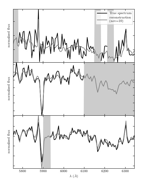
Figure 7.7
The principal component vectors defined for the SDSS spectra can be used to interpolate across or reconstruct missing data. Examples of three masked spectral regions are shown comparing the reconstruction of the input spectrum (black line) using the mean and the first ten eigenspectra (blue line) The gray bands represent the masked region of the spectrum.
# Author: Jake VanderPlas
# License: BSD
#   The figure produced by this code is published in the textbook
#   "Statistics, Data Mining, and Machine Learning in Astronomy" (2013)
#   For more information, see http://astroML.github.com
#   To report a bug or issue, use the following forum:
#    https://groups.google.com/forum/#!forum/astroml-general
import numpy as np
from matplotlib import pyplot as plt
from matplotlib import ticker

from astroML.datasets import fetch_sdss_corrected_spectra
from astroML.datasets import sdss_corrected_spectra

#----------------------------------------------------------------------
# This function adjusts matplotlib settings for a uniform feel in the textbook.
# Note that with usetex=True, fonts are rendered with LaTeX.  This may
# result in an error if LaTeX is not installed on your system.  In that case,
# you can set usetex to False.
if "setup_text_plots" not in globals():
    from astroML.plotting import setup_text_plots
setup_text_plots(fontsize=8, usetex=True)

#------------------------------------------------------------
# Get spectra and eigenvectors used to reconstruct them
data = fetch_sdss_corrected_spectra()
spec = sdss_corrected_spectra.reconstruct_spectra(data)
lam = sdss_corrected_spectra.compute_wavelengths(data)
evecs = data['evecs']
mu = data['mu']
norms = data['norms']
mask = data['mask']

#------------------------------------------------------------
# plot the results
i_plot = ((lam > 5750) & (lam < 6350))
lam = lam[i_plot]

specnums = [20, 8, 9]
subplots = [311, 312, 313]

fig = plt.figure(figsize=(5, 6.25))
fig.subplots_adjust(left=0.09, bottom=0.08, hspace=0, right=0.92, top=0.95)

for subplot, i in zip(subplots, specnums):
    ax = fig.add_subplot(subplot)

    # compute eigen-coefficients
    spec_i_centered = spec[i] / norms[i] - mu
    coeffs = np.dot(spec_i_centered, evecs.T)

    # blank out masked regions
    spec_i = spec[i]
    mask_i = mask[i]
    spec_i[mask_i] = np.nan

    # plot the raw masked spectrum
    ax.plot(lam, spec_i[i_plot], '-', color='k',
            label='True spectrum', lw=1.5)

    # plot two levels of reconstruction
    for nev in [10]:
        if nev == 0:
            label = 'mean'
        else:
            label = 'reconstruction\n(nev=%i)' % nev
        spec_i_recons = norms[i] * (mu + np.dot(coeffs[:nev], evecs[:nev]))
        ax.plot(lam, spec_i_recons[i_plot], label=label, color='grey')

    # plot shaded background in masked region
    ylim = ax.get_ylim()
    mask_shade = ylim[0] + mask[i][i_plot].astype(float) * ylim[1]
    plt.fill(np.concatenate([lam[:1], lam, lam[-1:]]),
             np.concatenate([[ylim[0]], mask_shade, [ylim[0]]]),
             lw=0, fc='k', alpha=0.2)

    ax.set_xlim(lam[0], lam[-1])
    ax.set_ylim(ylim)
    ax.yaxis.set_major_formatter(ticker.NullFormatter())

    if subplot == 311:
        ax.legend(loc=1)

    ax.set_xlabel('$\lambda\ (\AA)$')
    ax.set_ylabel('normalized flux')

plt.show()