Histogram vs Kernel Density Estimation
Figure 6.1
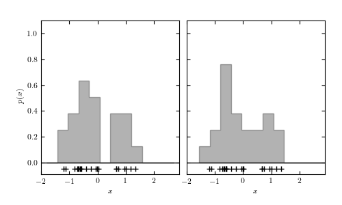
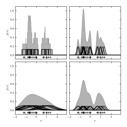
Density estimation using histograms and kernels. The top panels show two histogram representations of the same data (shown by plus signs in the bottom of each panel) using the same bin width, but with the bin centers of the histograms offset by 0.25. The middle-left panel shows an adaptive histogram where each bin is centered on an individual point and these bins can overlap. This adaptive representation preserves the bimodality of the data. The remaining panels show kernel density estimation using Gaussian kernels with different bandwidths, increasing from the middle-right panel to the bottom-right, and with the largest bandwidth in the bottom-left panel. The trade-off of variance for bias becomes apparent as the bandwidth of the kernels increases.
# Author: Jake VanderPlas
# License: BSD
#   The figure produced by this code is published in the textbook
#   "Statistics, Data Mining, and Machine Learning in Astronomy" (2013)
#   For more information, see http://astroML.github.com
#   To report a bug or issue, use the following forum:
#    https://groups.google.com/forum/#!forum/astroml-general
import numpy as np
from matplotlib import pyplot as plt
from scipy import stats

#----------------------------------------------------------------------
# This function adjusts matplotlib settings for a uniform feel in the textbook.
# Note that with usetex=True, fonts are rendered with LaTeX.  This may
# result in an error if LaTeX is not installed on your system.  In that case,
# you can set usetex to False.
if "setup_text_plots" not in globals():
    from astroML.plotting import setup_text_plots
setup_text_plots(fontsize=8, usetex=True)

#------------------------------------------------------------
# Draw the random data
np.random.seed(1)
x = np.concatenate([np.random.normal(-0.5, 0.3, size=14),
                    np.random.normal(1, 0.3, size=7)])


#------------------------------------------------------------
# First figure: silly histogram binning
fig1 = plt.figure(figsize=(5, 3))
fig1.subplots_adjust(left=0.12, right=0.95, wspace=0.05,
                     bottom=0.15, top=0.9, hspace=0.05)

FC = '#6666FF'
XLIM = (-2, 2.9)
YLIM = (-0.09, 1.1)

ax = fig1.add_subplot(121)
bins = np.linspace(-1.8, 2.7, 13)
ax.hist(x, bins=bins, density=True,
        histtype='stepfilled', fc='k', alpha=0.3)
ax.plot(XLIM, [0, 0], '-k', lw=1)
ax.plot(x, 0 * x - 0.05, '+k')
ax.set_xlim(XLIM)
ax.set_ylim(YLIM)
ax.set_xlabel('$x$')
ax.set_ylabel('$p(x)$')

ax = fig1.add_subplot(122)
ax.yaxis.set_major_formatter(plt.NullFormatter())
ax.hist(x, bins=bins + 0.25, density=True,
        histtype='stepfilled', fc='k', alpha=0.3)
ax.plot(XLIM, [0, 0], '-k', lw=1)
ax.plot(x, 0 * x - 0.05, '+k')
ax.set_xlim(XLIM)
ax.set_ylim(YLIM)
ax.set_xlabel('$x$')

#------------------------------------------------------------
# First figure: transition to KDE
fig2 = plt.figure(figsize=(5, 5))
fig2.subplots_adjust(left=0.12, right=0.95, wspace=0.05,
                     bottom=0.1, top=0.95, hspace=0.05)

ax = fig2.add_subplot(221)
ax.xaxis.set_major_formatter(plt.NullFormatter())
binwidth = bins[1] - bins[0]
x_plot = np.linspace(-4, 4, 1000)
y_plot = (abs(x_plot - x[:, None]) <= 0.5 * binwidth).astype(float)
y_plot /= (binwidth * len(x))
ax.fill(x_plot, y_plot.sum(0), ec='k', lw=1, fc='k', alpha=0.3)
ax.plot(x_plot, y_plot.T, '-k', lw=1)
ax.plot(x, 0 * x - 0.05, '+k')
ax.set_xlim(XLIM)
ax.set_ylim(YLIM)
ax.set_ylabel('$p(x)$')

ax = fig2.add_subplot(222)
ax.xaxis.set_major_formatter(plt.NullFormatter())
ax.yaxis.set_major_formatter(plt.NullFormatter())
binwidth = bins[1] - bins[0]
x_plot = np.linspace(-4, 4, 1000)
y_plot = binwidth * stats.norm.pdf(x_plot, x[:, None], 0.1)
y_plot /= (binwidth * len(x))
ax.fill(x_plot, y_plot.sum(0), ec='k', lw=1, fc='k', alpha=0.3)
ax.plot(x_plot, y_plot.T, '-k', lw=1)
ax.plot(x, 0 * x - 0.05, '+k')
ax.set_xlim(XLIM)
ax.set_ylim(YLIM)

ax = fig2.add_subplot(223)
binwidth = bins[1] - bins[0]
x_plot = np.linspace(-4, 4, 1000)
y_plot = binwidth * stats.norm.pdf(x_plot, x[:, None], 0.7)
y_plot /= (binwidth * len(x))
ax.fill(x_plot, y_plot.sum(0), ec='k', lw=1, fc='k', alpha=0.3)
ax.plot(x_plot, 4 * y_plot.T, '-k', lw=1)
ax.plot(x, 0 * x - 0.05, '+k')
ax.set_xlim(XLIM)
ax.set_ylim(YLIM)
ax.set_ylabel('$p(x)$')
ax.set_xlabel('$x$')

ax = fig2.add_subplot(224)
ax.yaxis.set_major_formatter(plt.NullFormatter())
binwidth = bins[1] - bins[0]
x_plot = np.linspace(-4, 4, 1000)
y_plot = binwidth * stats.norm.pdf(x_plot, x[:, None], 0.2)
y_plot /= (binwidth * len(x))
ax.fill(x_plot, y_plot.sum(0), ec='k', lw=1, fc='k', alpha=0.3)
ax.plot(x_plot, y_plot.T, '-k', lw=1)
ax.plot(x, 0 * x - 0.05, '+k')
ax.set_xlim(XLIM)
ax.set_ylim(YLIM)
ax.set_xlabel('$x$')

plt.show()