Posterior for Cauchy Distribution

Figure 5.11

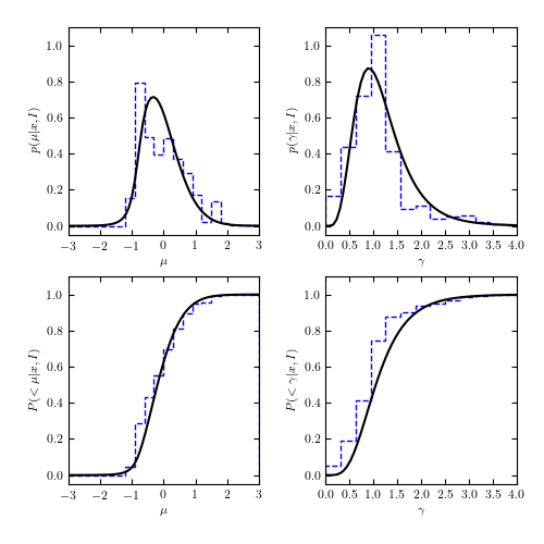
The solid lines show the posterior pdf (top-left panel) and the posterior pdf (top-right panel) for the two-dimensional pdf from figure 5.10. The dashed lines show the distribution of approximate estimates of and based on the median and interquartile range. The bottom panels show the corresponding cumulative distributions.

Code output:

Python source code:

# Author: Jake VanderPlas
# License: BSD
#   The figure produced by this code is published in the textbook
#   "Statistics, Data Mining, and Machine Learning in Astronomy" (2013)
#   For more information, see http://astroML.github.com
#   To report a bug or issue, use the following forum:
#    https://groups.google.com/forum/#!forum/astroml-general
import numpy as np
from matplotlib import pyplot as plt
from scipy.stats import cauchy
from astroML.stats import median_sigmaG
from astroML.resample import bootstrap

#----------------------------------------------------------------------
# This function adjusts matplotlib settings for a uniform feel in the textbook.
# Note that with usetex=True, fonts are rendered with LaTeX.  This may
# result in an error if LaTeX is not installed on your system.  In that case,
# you can set usetex to False.
if "setup_text_plots" not in globals():
    from astroML.plotting import setup_text_plots
setup_text_plots(fontsize=8, usetex=True)


def cauchy_logL(x, gamma, mu):
    """Equation 5.74: cauchy likelihood"""
    x = np.asarray(x)
    n = x.size

    # expand x for broadcasting
    shape = np.broadcast(gamma, mu).shape
    x = x.reshape(x.shape + tuple([1 for s in shape]))

    return ((n - 1) * np.log(gamma)
            - np.sum(np.log(gamma ** 2 + (x - mu) ** 2), 0))


def estimate_mu_gamma(xi, axis=None):
    """Equation 3.54: Cauchy point estimates"""
    q25, q50, q75 = np.percentile(xi, [25, 50, 75], axis=axis)
    return q50, 0.5 * (q75 - q25)


#------------------------------------------------------------
# Draw a random sample from the cauchy distribution, and compute
# marginalized posteriors of mu and gamma
np.random.seed(44)

n = 10
mu_0 = 0
gamma_0 = 2
xi = cauchy(mu_0, gamma_0).rvs(n)

gamma = np.linspace(0.01, 5, 70)
dgamma = gamma[1] - gamma[0]

mu = np.linspace(-3, 3, 70)
dmu = mu[1] - mu[0]

likelihood = np.exp(cauchy_logL(xi, gamma[:, np.newaxis], mu))

pmu = likelihood.sum(0)
pmu /= pmu.sum() * dmu

pgamma = likelihood.sum(1)
pgamma /= pgamma.sum() * dgamma

#------------------------------------------------------------
# bootstrap estimate
mu_bins = np.linspace(-3, 3, 21)
gamma_bins = np.linspace(0, 5, 17)

mu_bootstrap, gamma_bootstrap = bootstrap(xi, 20000, estimate_mu_gamma,
                                          kwargs=dict(axis=1), random_state=0)

#------------------------------------------------------------
# Plot results
fig = plt.figure(figsize=(5, 5))
fig.subplots_adjust(wspace=0.35, right=0.95,
                    hspace=0.2, top=0.95)

# first axes: mu posterior
ax1 = fig.add_subplot(221)
ax1.plot(mu, pmu, '-k')
ax1.hist(mu_bootstrap, mu_bins, density=True,
         histtype='step', color='b', linestyle='dashed')
ax1.set_xlabel(r'$\mu$')
ax1.set_ylabel(r'$p(\mu|x,I)$')

# second axes: mu cumulative posterior
ax2 = fig.add_subplot(223, sharex=ax1)
ax2.plot(mu, pmu.cumsum() * dmu, '-k')
ax2.hist(mu_bootstrap, mu_bins, density=True, cumulative=True,
         histtype='step', color='b', linestyle='dashed')
ax2.set_xlabel(r'$\mu$')
ax2.set_ylabel(r'$P(<\mu|x,I)$')
ax2.set_xlim(-3, 3)

# third axes: gamma posterior
ax3 = fig.add_subplot(222, sharey=ax1)
ax3.plot(gamma, pgamma, '-k')
ax3.hist(gamma_bootstrap, gamma_bins, density=True,
         histtype='step', color='b', linestyle='dashed')
ax3.set_xlabel(r'$\gamma$')
ax3.set_ylabel(r'$p(\gamma|x,I)$')
ax3.set_ylim(-0.05, 1.1)

# fourth axes: gamma cumulative posterior
ax4 = fig.add_subplot(224, sharex=ax3, sharey=ax2)
ax4.plot(gamma, pgamma.cumsum() * dgamma, '-k')
ax4.hist(gamma_bootstrap, gamma_bins, density=True, cumulative=True,
         histtype='step', color='b', linestyle='dashed')
ax4.set_xlabel(r'$\gamma$')
ax4.set_ylabel(r'$P(<\gamma|x,I)$')
ax4.set_ylim(-0.05, 1.1)
ax4.set_xlim(0, 4)

plt.show()

[download source: fig_posterior_cauchy.py]