Plot the Outlier Probability
Figure 5.18
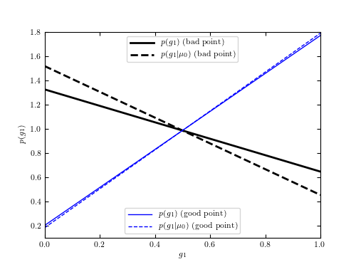
The marginal probability for g_i for the “good” and “bad” points shown in
figure 5.17. The solid curves show the marginalized probability: that is,
eq. 5.100 is integrated over mu. The dashed curves show the probability
conditioned on  , the MAP estimate of
  (eq. 5.102)
# Author: Jake VanderPlas
# License: BSD
#   The figure produced by this code is published in the textbook
#   "Statistics, Data Mining, and Machine Learning in Astronomy" (2013)
#   For more information, see http://astroML.github.com
#   To report a bug or issue, use the following forum:
#    https://groups.google.com/forum/#!forum/astroml-general
import numpy as np
from matplotlib import pyplot as plt
from scipy.stats import norm

#----------------------------------------------------------------------
# This function adjusts matplotlib settings for a uniform feel in the textbook.
# Note that with usetex=True, fonts are rendered with LaTeX.  This may
# result in an error if LaTeX is not installed on your system.  In that case,
# you can set usetex to False.
if "setup_text_plots" not in globals():
    from astroML.plotting import setup_text_plots
setup_text_plots(fontsize=8, usetex=True)


def p(mu, g1, xi, sigma1, sigma2):
    """Equation 5.97: marginalized likelihood over outliers"""
    L = (g1 * norm.pdf(xi[0], mu, sigma1) +
         (1 - g1) * norm.pdf(xi[0], mu, sigma2))

    mu = mu.reshape(mu.shape + (1,))
    g1 = g1.reshape(g1.shape + (1,))

    return L * np.prod(norm.pdf(xi[1:], mu, sigma1)
                       + norm.pdf(xi[1:], mu, sigma2), -1)

#------------------------------------------------------------
# Sample the points
np.random.seed(138)

N1 = 8
N2 = 2
sigma1 = 1
sigma2 = 3

sigmai = np.zeros(N1 + N2)
sigmai[N2:] = sigma1
sigmai[:N2] = sigma2

xi = np.random.normal(0, sigmai)

#------------------------------------------------------------
# Compute the marginalized posterior for the first and last point
mu = np.linspace(-5, 5, 71)
g1 = np.linspace(0, 1, 71)

L1 = p(mu[:, None], g1, xi, 1, 10)
L1 /= np.max(L1)

(i1, j1) = np.where(L1 == 1)
mu0_1 = mu[i1]


L2 = p(mu[:, None], g1, xi[::-1], 1, 10)
L2 /= np.max(L2)
(i2, j2) = np.where(L2 == 1)
mu0_2 = mu[i2]

p1 = L1.sum(0)
p2 = L2.sum(0)

p1 /= np.sum(p1) * (g1[1] - g1[0])
p2 /= np.sum(p2) * (g1[1] - g1[0])

p1a = L1[i1[0]]
p2a = L2[i2[0]]

p1a /= p1a.sum() * (g1[1] - g1[0])
p2a /= p2a.sum() * (g1[1] - g1[0])

#------------------------------------------------------------
# Plot the results
fig, ax = plt.subplots(figsize=(5, 3.75))

l1, = ax.plot(g1, p1, '-k', lw=2)
l2, = ax.plot(g1, p1a, '--k', lw=2)
leg1 = ax.legend([l1, l2],
                 [r'$p(g_1)$ (bad point)',
                  r'$p(g_1|\mu_0)$ (bad point)'], loc=9)

l3, = ax.plot(g1, p2, '-b', lw=1, label=r'$p(g_1)$ (good point)')
l4, = ax.plot(g1, p2a, '--b', lw=1, label=r'$p(g_1|\mu_0)$ (good point)')
leg2 = ax.legend([l3, l4],
                 [r'$p(g_1)$ (good point)',
                  r'$p(g_1|\mu_0)$ (good point)'], loc=8)

# trick to display two legends:
# when legend() is called the second time, the first one is removed from
# the axes.  We add it back in here:
ax.add_artist(leg1)

ax.set_xlabel('$g_1$')
ax.set_ylabel('$p(g_1)$')

ax.set_xlim(0, 1)
ax.set_ylim(0.1, 1.8)

plt.show()