Log-likelihood for Gaussian plus linear background

Figure 5.13

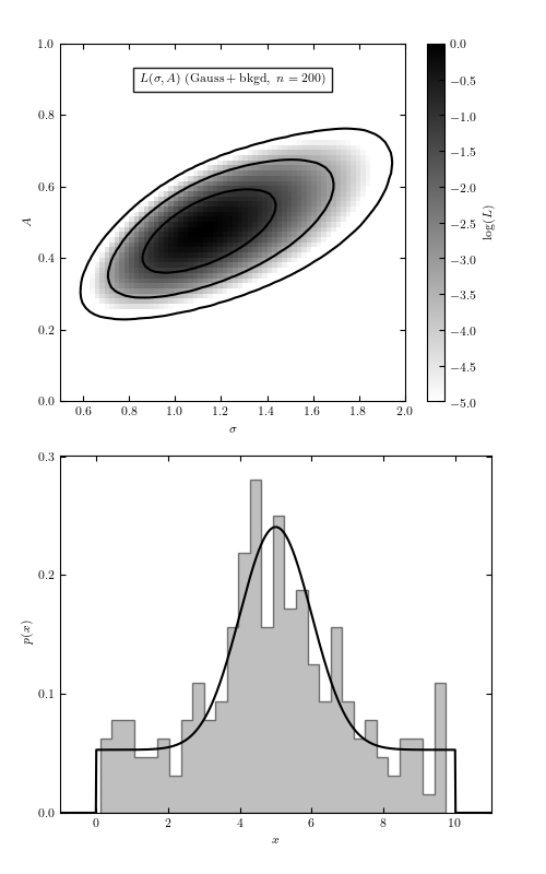
An illustration of the logarithm of the posterior probability density function (see eq. 5.85) for data generated using N = 200, , , and A = 0.5, with the background strength (1 - A)/W = 0.05 in the interval 0 < x < W, W = 10. The maximum of is renormalized to 0, and color coded on a scale -5 to 0, as shown in the legend. The contours enclose the regions that contain 0.683, 0.955, and 0.997 of the cumulative (integrated) posterior probability. Note the covariance between A and . The histogram in the bottom panel shows the distribution of data values used to construct the posterior pdf in the top panel, and the probability density function from which the data were drawn as the solid line.

Code output:

Python source code:

# Author: Jake VanderPlas
# License: BSD
#   The figure produced by this code is published in the textbook
#   "Statistics, Data Mining, and Machine Learning in Astronomy" (2013)
#   For more information, see http://astroML.github.com
#   To report a bug or issue, use the following forum:
#    https://groups.google.com/forum/#!forum/astroml-general
import numpy as np
from matplotlib import pyplot as plt
from scipy.stats import truncnorm, uniform
from astroML.plotting.mcmc import convert_to_stdev

#----------------------------------------------------------------------
# This function adjusts matplotlib settings for a uniform feel in the textbook.
# Note that with usetex=True, fonts are rendered with LaTeX.  This may
# result in an error if LaTeX is not installed on your system.  In that case,
# you can set usetex to False.
if "setup_text_plots" not in globals():
    from astroML.plotting import setup_text_plots
setup_text_plots(fontsize=8, usetex=True)


def gausslin_logL(xi, A=0.5, sigma=1.0, mu=5.0, L=10.0):
    """Equation 5.80: gaussian likelihood with uniform background"""
    xi = np.asarray(xi)

    shape = np.broadcast(sigma, A, mu, L).shape

    xi = xi.reshape(xi.shape + tuple([1 for s in shape]))

    return np.sum(np.log(A * np.exp(-0.5 * ((xi - mu) / sigma) ** 2)
                         / (sigma * np.sqrt(2 * np.pi))
                         + (1. - A) / L), 0)

#------------------------------------------------------------
# Define the distribution
np.random.seed(0)
mu = 5.0
sigma = 1.0
L = 10.0
A = 0.5
N = 200

xi = np.random.random(N)
NA = np.sum(xi < A)

dist1 = truncnorm((0 - mu) / sigma, (L - mu) / sigma, mu, sigma)
dist2 = uniform(0, 10)

xi[:NA] = dist1.rvs(NA)
xi[NA:] = dist2.rvs(N - NA)

x = np.linspace(-1, 11, 1000)
fracA = NA * 1. / N

#------------------------------------------------------------
# define the (sigma, A) grid and compute logL
sigma = np.linspace(0.5, 2, 70)
A = np.linspace(0, 1, 70)

logL = gausslin_logL(xi, A[:, np.newaxis], sigma)
logL -= logL.max()

#------------------------------------------------------------
# Plot the results
fig = plt.figure(figsize=(5, 8))
fig.subplots_adjust(bottom=0.07, left=0.11, hspace=0.15, top=0.95)

ax = fig.add_subplot(211)
plt.imshow(logL, origin='lower', aspect='auto',
           extent=(sigma[0], sigma[-1], A[0], A[-1]),
           cmap=plt.cm.binary)
plt.colorbar().set_label(r'$\log(L)$')
plt.clim(-5, 0)
ax.set_xlabel(r'$\sigma$')
ax.set_ylabel(r'$A$')

ax.text(0.5, 0.9, r'$L(\sigma,A)\ (\mathrm{Gauss + bkgd},\ n=200)$',
        bbox=dict(ec='k', fc='w', alpha=0.9),
        ha='center', va='center', transform=plt.gca().transAxes)

ax.contour(sigma, A, convert_to_stdev(logL),
           levels=(0.683, 0.955, 0.997),
           colors='k')

ax2 = plt.subplot(212)
ax2.yaxis.set_major_locator(plt.MultipleLocator(0.1))
ax2.plot(x, fracA * dist1.pdf(x) + (1. - fracA) * dist2.pdf(x), '-k')
ax2.hist(xi, 30, density=True, histtype='stepfilled', fc='gray', alpha=0.5)

ax2.set_ylim(0, 0.301)
ax2.set_xlim(-1, 11)

ax2.set_xlabel('$x$')
ax2.set_ylabel('$p(x)$')
plt.show()

[download source: fig_likelihood_gausslin.py]