Approximate Bayesian Computation for Gaussian location parameter
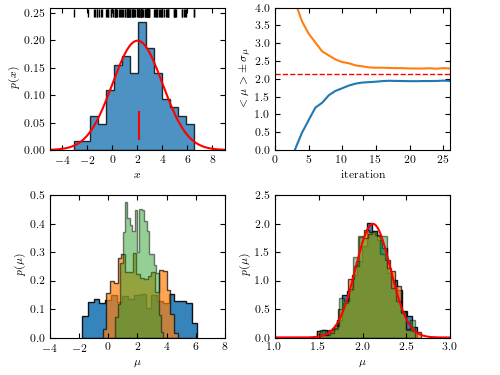
Figure 5.29 An example of Approximate Bayesian Computation: estimate the location parameter for a sample drawn from Gaussian distribution with known scale parameter.
iteration: 1
iteration: 2
iteration: 3
iteration: 4
iteration: 5
iteration: 6
iteration: 7
iteration: 8
iteration: 9
iteration: 10
iteration: 11
iteration: 12
iteration: 13
iteration: 14
iteration: 15
iteration: 16
iteration: 17
iteration: 18
iteration: 19
iteration: 20
iteration: 21
iteration: 22
iteration: 23
iteration: 24
iteration: 25
# Author: Zeljko Ivezic
# License: BSD
#   The figure produced by this code is published in the textbook
#   "Statistics, Data Mining, and Machine Learning in Astronomy" (2019)
#   For more information, see http://astroML.github.com
#   To report a bug or issue, use the following forum:
#    https://groups.google.com/forum/#!forum/astroml-general
import numpy as np
from matplotlib import pyplot as plt
from scipy.stats import norm

#----------------------------------------------------------------------
# This function adjusts matplotlib settings for a uniform feel in the textbook.
# Note that with usetex=True, fonts are rendered with LaTeX.  This may
# result in an error if LaTeX is not installed on your system. In that case,
# you can set usetex to False.
from astroML.plotting import setup_text_plots
setup_text_plots(fontsize=8, usetex=True)


def plotABC(theta, weights, Niter, data, muTrue, sigTrue):

    Nresample = 100000
    Ndata = np.size(data)
    xmean = np.mean(data)
    sigPosterior = sigTrue / np.sqrt(Ndata)
    truedist = norm(xmean, sigPosterior)
    x = np.linspace(-10, 10, 1000)
    for j in range(0, Niter):
        meanT[j] = np.mean(theta[j])
        stdT[j] = np.std(theta[j])

    # plot
    fig = plt.figure(figsize=(5, 3.75))
    fig.subplots_adjust(left=0.1, right=0.95, wspace=0.24,
                        bottom=0.1, top=0.95)

    # last few iterations
    ax1 = fig.add_axes((0.55, 0.1, 0.35, 0.38))
    ax1.set_xlabel(r'$\mu$')
    ax1.set_ylabel(r'$p(\mu)$')
    ax1.set_xlim(1.0, 3.0)
    ax1.set_ylim(0, 2.5)
    for j in [15, 20, 25]:
        sample = weightedResample(theta[j], Nresample, weights[j])
        ax1.hist(sample, 20, density=True, histtype='stepfilled',
                 alpha=0.9-(0.04*(j-15)))
    ax1.plot(x, truedist.pdf(x), 'r')

    # first few iterations
    ax2 = fig.add_axes((0.1, 0.1, 0.35, 0.38))
    ax2.set_xlabel(r'$\mu$')
    ax2.set_ylabel(r'$p(\mu)$')
    ax2.set_xlim(-4.0, 8.0)
    ax2.set_ylim(0, 0.5)
    for j in [2, 4, 6]:
        sample = weightedResample(theta[j], Nresample, weights[j])
        ax2.hist(sample, 20, density=True, histtype='stepfilled',
                 alpha=(0.9-0.1*(j-2)))

    # mean and scatter vs. iteration number
    ax3 = fig.add_axes((0.55, 0.60, 0.35, 0.38))
    ax3.set_xlabel('iteration')
    ax3.set_ylabel(r'$<\mu> \pm \, \sigma_\mu$')
    ax3.set_xlim(0, Niter)
    ax3.set_ylim(0, 4)
    iter = np.linspace(1, Niter, Niter)
    meanTm = meanT - stdT
    meanTp = meanT + stdT
    ax3.plot(iter, meanTm)
    ax3.plot(iter, meanTp)
    ax3.plot([0, Niter], [xmean, xmean], ls="--", c="r", lw=1)

    # data
    ax4 = fig.add_axes((0.1, 0.60, 0.35, 0.38))
    ax4.set_xlabel(r'$x$')
    ax4.set_ylabel(r'$p(x)$')
    ax4.set_xlim(-5, 9)
    ax4.set_ylim(0, 0.26)
    ax4.hist(data, 15, density=True, histtype='stepfilled', alpha=0.8)
    datadist = norm(muTrue, sigTrue)
    ax4.plot(x, datadist.pdf(x), 'r')
    ax4.plot([xmean, xmean], [0.02, 0.07], c='r')
    ax4.plot(data, 0.25 * np.ones(len(data)), '|k')

    plt.show()


#----------------------------------------------------------------------
def distance(x, y):
    return np.abs(np.mean(x) - np.mean(y))


def weightedResample(x, N, weights):
    # resample N elements from x, with selection prob. proportional to weights
    p = weights / np.sum(weights)
    return np.random.choice(x, size=N, replace=True, p=p)


# return the kernel values
def kernelValues(prevThetas, prevStdDev, currentTheta):
    return norm(currentTheta, prevStdDev).pdf(prevThetas)


# return new values, scattered around an old value using kernel
def kernelSample(theta, stdDev, Nsample=1):
    return np.random.normal(theta, stdDev, Nsample)


# compute new weight
def computeWeight(prevWeights, prevThetas, prevStdDev, currentTheta):
    denom = prevWeights * kernelValues(prevThetas, prevStdDev, currentTheta)
    return prior(currentTheta, prevThetas) / np.sum(denom)


# flat prior probability
def prior(thisTheta, allThetas):
    return 1.0 / np.size(allThetas)


def getData(Ndata, mu, sigma):
    # use simulated data
    return simulateData(Ndata, mu, sigma)


def simulateData(Ndata, mu, sigma):
    # simple gaussian toy model
    return np.random.normal(mu, sigma, Ndata)


def KLscatter(x, w, N):
    sample = weightedResample(x, N, w)
    return np.sqrt(2) * np.std(sample)


#----------------------------------------------------------------------
np.random.seed(0)    # for repeatability

# "observed" data:
Ndata = 100
muTrue = 2.0
sigmaTrue = 2.0
data = getData(Ndata, muTrue, sigmaTrue)
dataMean = np.mean(data)
# conservative choice for initial tolerance
eps0 = np.max(data) - np.min(data)
# limits for uniform prior
thetaMin = -10
thetaMax = 10

# sampling parameters
Ndraw = 1000
Niter = 26
DpercCut = 80
theta = np.empty([Niter, Ndraw])
weights = np.empty([Niter, Ndraw])
D = np.empty([Niter, Ndraw])
eps = np.empty([Niter])
meanT = np.zeros(Niter)
stdT = np.zeros(Niter)

# first sample from uniform prior, draw samples and compute their distance to data
for i in range(0, Ndraw):
    thetaS = np.random.uniform(thetaMin, thetaMax)
    sample = simulateData(Ndata, thetaS, sigmaTrue)
    D[0][i] = distance(data, sample)
    theta[0][i] = thetaS

weights[0] = 1.0 / Ndraw
scatter = KLscatter(theta[0], weights[0], Ndraw)
eps[0] = np.percentile(D[0], 50)


# ABC iterations:
ssTot = 0
verbose = False

for j in range(1, Niter):
    print('iteration:', j)
    thetaOld = theta
    weightsOld = weights / np.sum(weights)
    # sample until distance condition fullfilled
    ss = 0
    for i in range(0, Ndraw):
        notdone = True
        while notdone:
            ss += 1
            ssTot += 1
            # sample from previous theta with probability given by weights: thetaS
            thetaS = weightedResample(theta[j-1], 1, weights[j-1])[0]
            # perturb thetaS with kernel
            thetaSS = kernelSample(thetaS, scatter)[0]
            # generate a simulated sample
            sample = simulateData(Ndata, thetaSS, sigmaTrue)
            dist = distance(data, sample)
            if (dist < eps[j-1]):
                notdone = False
        D[j][i] = dist
        theta[j][i] = thetaSS
        # get weight for new theta
        weights[j][i] = computeWeight(weights[j-1], theta[j-1], scatter, thetaSS)
    # new kernel scatter value
    scatter = KLscatter(theta[j], weights[j], Ndraw)
    eps[j] = np.percentile(D[j], DpercCut)
    if (verbose):
        print('         acceptance rate (%):', (100.0*Ndraw/ss))
        print('                 new epsilon:', eps[j])
        print('              sample scatter:', scatter)
if (verbose):
    print('number of simulation evaluations:', ssTot)
# plot
plotABC(theta, weights, Niter, data, muTrue, sigmaTrue)