Bivariate Gaussian
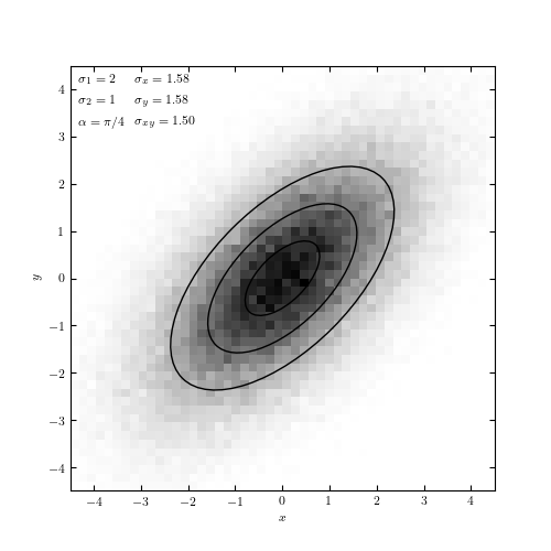
Figure 3.22.
An example of data generated from a bivariate Gaussian distribution. The shaded pixels are a Hess diagram showing the density of points at each position.
# Author: Jake VanderPlas
# License: BSD
#   The figure produced by this code is published in the textbook
#   "Statistics, Data Mining, and Machine Learning in Astronomy" (2013)
#   For more information, see http://astroML.github.com
#   To report a bug or issue, use the following forum:
#    https://groups.google.com/forum/#!forum/astroml-general
import numpy as np
from matplotlib import pyplot as plt
from matplotlib.patches import Ellipse
from astroML.stats.random import bivariate_normal

#----------------------------------------------------------------------
# This function adjusts matplotlib settings for a uniform feel in the textbook.
# Note that with usetex=True, fonts are rendered with LaTeX.  This may
# result in an error if LaTeX is not installed on your system.  In that case,
# you can set usetex to False.
if "setup_text_plots" not in globals():
    from astroML.plotting import setup_text_plots
setup_text_plots(fontsize=8, usetex=True)

#------------------------------------------------------------
# Define the mean, principal axes, and rotation of the ellipse
mean = np.array([0, 0])
sigma_1 = 2
sigma_2 = 1
alpha = np.pi / 4

#------------------------------------------------------------
# Draw 10^5 points from a multivariate normal distribution
#
#   we use the bivariate_normal function from astroML.  A more
#   general function for this is numpy.random.multivariate_normal(),
#   which requires the user to specify the full covariance matrix.
#   bivariate_normal() generates this covariance matrix for the
#   given inputs.
np.random.seed(0)
x, cov = bivariate_normal(mean, sigma_1, sigma_2, alpha, size=100000,
                          return_cov=True)

sigma_x = np.sqrt(cov[0, 0])
sigma_y = np.sqrt(cov[1, 1])
sigma_xy = cov[0, 1]

#------------------------------------------------------------
# Plot the results
fig = plt.figure(figsize=(5, 5))
ax = fig.add_subplot(111)

# plot a 2D histogram/hess diagram of the points
H, bins = np.histogramdd(x, bins=2 * [np.linspace(-4.5, 4.5, 51)])
ax.imshow(H, origin='lower', cmap=plt.cm.binary, interpolation='nearest',
          extent=[bins[0][0], bins[0][-1], bins[1][0], bins[1][-1]])

# draw 1, 2, 3-sigma ellipses over the distribution
for N in (1, 2, 3):
    ax.add_patch(Ellipse(mean, N * sigma_1, N * sigma_2,
                         angle=alpha * 180. / np.pi, lw=1,
                         ec='k', fc='none'))

kwargs = dict(ha='left', va='top', transform=ax.transAxes)

ax.text(0.02, 0.98, r"$\sigma_1 = %i$" % sigma_1, **kwargs)
ax.text(0.02, 0.93, r"$\sigma_2 = %i$" % sigma_2, **kwargs)
ax.text(0.02, 0.88, r"$\alpha = \pi / %i$" % (np.pi / alpha), **kwargs)

ax.text(0.15, 0.98, r"$\sigma_x = %.2f$" % sigma_x, **kwargs)
ax.text(0.15, 0.93, r"$\sigma_y = %.2f$" % sigma_y, **kwargs)
ax.text(0.15, 0.88, r"$\sigma_{xy} = %.2f$" % sigma_xy, **kwargs)

ax.set_xlabel('$x$')
ax.set_ylabel('$y$')

plt.show()