Search Algorithm Scaling

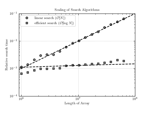
Figure 2.1.

The scaling of two methods to search for an item in an ordered list: a linear method which performs a comparison on all N items, and a binary search which uses a more sophisticated algorithm. The theoretical scalings are shown by dashed lines.

Code output:

Python source code:

# Author: Jake VanderPlas
# License: BSD
#   The figure produced by this code is published in the textbook
#   "Statistics, Data Mining, and Machine Learning in Astronomy" (2013)
#   For more information, see http://astroML.github.com
#   To report a bug or issue, use the following forum:
#    https://groups.google.com/forum/#!forum/astroml-general
from time import time
import numpy as np
from matplotlib import pyplot as plt

#----------------------------------------------------------------------
# This function adjusts matplotlib settings for a uniform feel in the textbook.
# Note that with usetex=True, fonts are rendered with LaTeX.  This may
# result in an error if LaTeX is not installed on your system.  In that case,
# you can set usetex to False.
if "setup_text_plots" not in globals():
    from astroML.plotting import setup_text_plots
setup_text_plots(fontsize=8, usetex=True)

#------------------------------------------------------------
# Compute the execution times as a function of array size
Nsamples = 10 ** np.linspace(6.0, 7.8, 17)
time_linear = np.zeros_like(Nsamples)
time_binary = np.zeros_like(Nsamples)

for i in range(len(Nsamples)):
    # create a sorted array
    x = np.arange(Nsamples[i], dtype=int)

    # Linear search: choose a single item in the array
    item = int(0.4 * Nsamples[i])

    t0 = time()
    j = np.where(x == item)
    t1 = time()

    time_linear[i] = t1 - t0

    # Binary search: this is much faster, so choose 1000 items to search for
    items = np.linspace(0, Nsamples[i], 1000).astype(int)

    t0 = time()
    j = np.searchsorted(x, items)
    t1 = time()

    time_binary[i] = (t1 - t0)

#------------------------------------------------------------
# Plot the results
fig = plt.figure(figsize=(5, 3.75))
fig.subplots_adjust(bottom=0.15)
ax = plt.axes(xscale='log', yscale='log')
ax.grid()

# plot the observed times
ax.plot(Nsamples, time_linear, 'ok', color='gray', markersize=5,
        label=r'linear search $(\mathcal{O}[N])$')
ax.plot(Nsamples, time_binary, 'sk', color='gray', markersize=5,
        label=r'efficient search $(\mathcal{O}[\log N])$')

# plot the expected scaling
scale = 10 ** np.linspace(5, 8, 100)
scaling_N = scale * time_linear[7] / Nsamples[7]
scaling_logN = np.log(scale) * time_binary[7] / np.log(Nsamples[7])
ax.plot(scale, scaling_N, '--k')
ax.plot(scale, scaling_logN, '--k')

ax.set_xlim(9E5, 1E8)

# add text and labels
ax.set_title("Scaling of Search Algorithms")
ax.set_xlabel('Length of Array')
ax.set_ylabel('Relative search time')
ax.legend(loc='upper left')

plt.show()

[download source: fig_search_scaling.py]