Wiener Filter / kernel smooting Connection
Figure 10.11
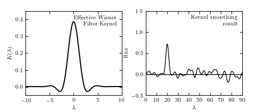
The left panel shows the inverse Fourier transform of the Wiener filter Phi(f) applied in figure 10.10. By the convolution theorem, the Wiener-filtered result is equivalent to the convolution of the unfiltered signal with the kernel shown above, and thus Wiener filtering and kernel smoothing are directly related. The right panel shows the data smoothed by this kernel, which is equivalent to the Wiener filter smoothing in figure 10.10.
# Author: Jake VanderPlas
# License: BSD
#   The figure produced by this code is published in the textbook
#   "Statistics, Data Mining, and Machine Learning in Astronomy" (2013)
#   For more information, see http://astroML.github.com
#   To report a bug or issue, use the following forum:
#    https://groups.google.com/forum/#!forum/astroml-general
import numpy as np
from matplotlib import pyplot as plt

from scipy import optimize, fftpack, interpolate
from astroML.fourier import IFT_continuous
from astroML.filters import wiener_filter

#----------------------------------------------------------------------
# This function adjusts matplotlib settings for a uniform feel in the textbook.
# Note that with usetex=True, fonts are rendered with LaTeX.  This may
# result in an error if LaTeX is not installed on your system.  In that case,
# you can set usetex to False.
if "setup_text_plots" not in globals():
    from astroML.plotting import setup_text_plots
setup_text_plots(fontsize=8, usetex=True)

#----------------------------------------------------------------------
# sample the same data as the previous Wiener filter figure
np.random.seed(5)
t = np.linspace(0, 100, 2001)[:-1]
h = np.exp(-0.5 * ((t - 20.) / 1.0) ** 2)
hN = h + np.random.normal(0, 0.5, size=h.shape)

#----------------------------------------------------------------------
# compute the PSD
N = len(t)
Df = 1. / N / (t[1] - t[0])
f = fftpack.ifftshift(Df * (np.arange(N) - N / 2))

h_wiener, PSD, P_S, P_N, Phi = wiener_filter(t, hN, return_PSDs=True)

#------------------------------------------------------------
# inverse fourier transform Phi to find the effective kernel
t_plot, kernel = IFT_continuous(f, Phi)

#------------------------------------------------------------
# perform kernel smoothing on the data.  This is faster in frequency
# space (ie using the standard Wiener filter above) but we will do
# it in the slow & simple way here to demonstrate the equivalence
# explicitly
kernel_func = interpolate.interp1d(t_plot, kernel.real)

t_eval = np.linspace(0, 90, 1000)
t_KDE = t_eval[:, np.newaxis] - t
t_KDE[t_KDE < t_plot[0]] = t_plot[0]
t_KDE[t_KDE > t_plot[-1]] = t_plot[-1]
F = kernel_func(t_KDE)

h_smooth = np.dot(F, hN) / np.sum(F, 1)

#------------------------------------------------------------
# Plot the results
fig = plt.figure(figsize=(5, 2.2))
fig.subplots_adjust(left=0.1, right=0.95, wspace=0.25,
                    bottom=0.15, top=0.9)

# First plot: the equivalent Kernel to the WF
ax = fig.add_subplot(121)
ax.plot(t_plot, kernel.real, '-k')
ax.text(0.95, 0.95, "Effective Wiener\nFilter Kernel",
        ha='right', va='top', transform=ax.transAxes)

ax.set_xlim(-10, 10)
ax.set_ylim(-0.05, 0.45)
ax.set_xlabel(r'$\lambda$')
ax.set_ylabel(r'$K(\lambda)$')

# Second axes: Kernel smoothed results
ax = fig.add_subplot(122)
ax.plot(t_eval, h_smooth, '-k', lw=1)
ax.plot(t_eval, 0 * t_eval, '-k', lw=1)
ax.text(0.95, 0.95, "Kernel smoothing\nresult",
        ha='right', va='top', transform=ax.transAxes)

ax.set_xlim(0, 90)
ax.set_ylim(-0.5, 1.5)

ax.set_xlabel('$\lambda$')
ax.set_ylabel('flux')

plt.show()