Wavelet transform of Gaussian Noise
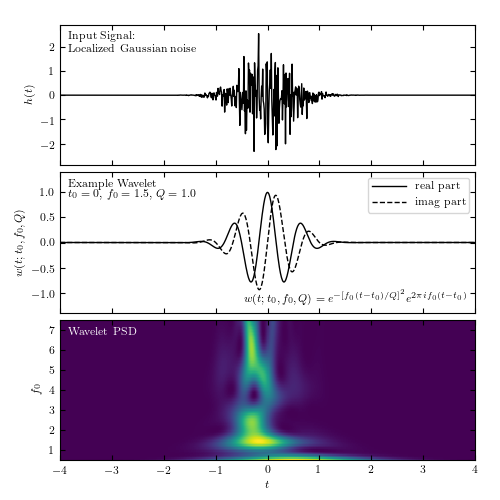
Figure 10.7
Localized frequency analysis using the wavelet transform. The upper panel shows the input signal, which consists of localized Gaussian noise. The middle panel shows an example wavelet. The lower panel shows the power spectral density as a function of the frequency f0 and the time t0, for Q = 1.0.
# Author: Jake VanderPlas
# License: BSD
#   The figure produced by this code is published in the textbook
#   "Statistics, Data Mining, and Machine Learning in Astronomy" (2013)
#   For more information, see http://astroML.github.com
#   To report a bug or issue, use the following forum:
#    https://groups.google.com/forum/#!forum/astroml-general
import numpy as np
from matplotlib import pyplot as plt

from astroML.fourier import\
    FT_continuous, IFT_continuous, sinegauss, sinegauss_FT, wavelet_PSD

#----------------------------------------------------------------------
# This function adjusts matplotlib settings for a uniform feel in the textbook.
# Note that with usetex=True, fonts are rendered with LaTeX.  This may
# result in an error if LaTeX is not installed on your system.  In that case,
# you can set usetex to False.
if "setup_text_plots" not in globals():
    from astroML.plotting import setup_text_plots
setup_text_plots(fontsize=8, usetex=True)

#------------------------------------------------------------
# Sample the function: localized noise
np.random.seed(0)

N = 1024
t = np.linspace(-5, 5, N)
x = np.ones(len(t))

h = np.random.normal(0, 1, len(t))
h *= np.exp(-0.5 * (t / 0.5) ** 2)

#------------------------------------------------------------
# Compute an example wavelet
W = sinegauss(t, 0, 1.5, Q=1.0)

#------------------------------------------------------------
# Compute the wavelet PSD
f0 = np.linspace(0.5, 7.5, 100)
wPSD = wavelet_PSD(t, h, f0, Q=1.0)

#------------------------------------------------------------
# Plot the results
fig = plt.figure(figsize=(5, 5))
fig.subplots_adjust(hspace=0.05, left=0.12, right=0.95, bottom=0.08, top=0.95)

# First panel: the signal
ax = fig.add_subplot(311)
ax.plot(t, h, '-k', lw=1)
ax.text(0.02, 0.95, ("Input Signal:\n"
                     "Localized Gaussian noise"),
        ha='left', va='top', transform=ax.transAxes)

ax.set_xlim(-4, 4)
ax.set_ylim(-2.9, 2.9)
ax.xaxis.set_major_formatter(plt.NullFormatter())
ax.set_ylabel('$h(t)$')

# Second panel: an example wavelet
ax = fig.add_subplot(312)
ax.plot(t, W.real, '-k', label='real part', lw=1)
ax.plot(t, W.imag, '--k', label='imag part', lw=1)

ax.text(0.02, 0.95, ("Example Wavelet\n"
                     "$t_0 = 0$, $f_0=1.5$, $Q=1.0$"),
        ha='left', va='top', transform=ax.transAxes)
ax.text(0.98, 0.05,
        (r"$w(t; t_0, f_0, Q) = e^{-[f_0 (t - t_0) / Q]^2}"
         "e^{2 \pi i f_0 (t - t_0)}$"),
        ha='right', va='bottom', transform=ax.transAxes)

ax.legend(loc=1)

ax.set_xlim(-4, 4)
ax.set_ylim(-1.4, 1.4)
ax.set_ylabel('$w(t; t_0, f_0, Q)$')
ax.xaxis.set_major_formatter(plt.NullFormatter())

# Third panel: the spectrogram
ax = plt.subplot(313)
ax.imshow(wPSD, origin='lower', aspect='auto',
          extent=[t[0], t[-1], f0[0], f0[-1]])

ax.text(0.02, 0.95, ("Wavelet PSD"), color='w',
        ha='left', va='top', transform=ax.transAxes)

ax.set_xlim(-4, 4)
ax.set_ylim(0.5, 7.5)

ax.set_xlabel('$t$')
ax.set_ylabel('$f_0$')

plt.show()