Generating Power-law Light Curves

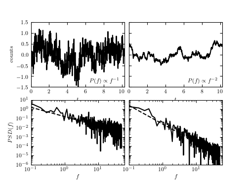
Figure 10.29

Examples of stochastic time series generated from power-law PSDs (left: 1/ f; right: 1/f^2) using the method from [1]. The top panels show the generated data, while the bottom panels show the corresponding PSD (dashed lines: input PSD; solid lines: determined from time series shown in the top panels).

References

1

Timmer, J. & Koenig, M. On Generating Power Law Noise. A&A 300:707

Code output:

Python source code:

# Author: Jake VanderPlas
# License: BSD
#   The figure produced by this code is published in the textbook
#   "Statistics, Data Mining, and Machine Learning in Astronomy" (2013)
#   For more information, see http://astroML.github.com
#   To report a bug or issue, use the following forum:
#    https://groups.google.com/forum/#!forum/astroml-general
import numpy as np
from matplotlib import pyplot as plt
from astroML.time_series import generate_power_law
from astroML.fourier import PSD_continuous

#----------------------------------------------------------------------
# This function adjusts matplotlib settings for a uniform feel in the textbook.
# Note that with usetex=True, fonts are rendered with LaTeX.  This may
# result in an error if LaTeX is not installed on your system.  In that case,
# you can set usetex to False.
if "setup_text_plots" not in globals():
    from astroML.plotting import setup_text_plots
setup_text_plots(fontsize=8, usetex=True)

N = 1024
dt = 0.01
factor = 100

t = dt * np.arange(N)
random_state = np.random.RandomState(1)

fig = plt.figure(figsize=(5, 3.75))
fig.subplots_adjust(wspace=0.05)

for i, beta in enumerate([1.0, 2.0]):
    # Generate the light curve and compute the PSD
    x = factor * generate_power_law(N, dt, beta, random_state=random_state)
    f, PSD = PSD_continuous(t, x)

    # First axes: plot the time series
    ax1 = fig.add_subplot(221 + i)
    ax1.plot(t, x, '-k')

    ax1.text(0.95, 0.05, r"$P(f) \propto f^{-%i}$" % beta,
             ha='right', va='bottom', transform=ax1.transAxes)

    ax1.set_xlim(0, 10.24)
    ax1.set_ylim(-1.5, 1.5)

    ax1.set_xlabel(r'$t$')

    # Second axes: plot the PSD
    ax2 = fig.add_subplot(223 + i, xscale='log', yscale='log')
    ax2.plot(f, PSD, '-k')
    ax2.plot(f[1:], (factor * dt) ** 2 * (2 * np.pi * f[1:]) ** -beta, '--k')

    ax2.set_xlim(1E-1, 60)
    ax2.set_ylim(1E-6, 1E1)

    ax2.set_xlabel(r'$f$')

    if i == 1:
        ax1.yaxis.set_major_formatter(plt.NullFormatter())
        ax2.yaxis.set_major_formatter(plt.NullFormatter())
    else:
        ax1.set_ylabel(r'${\rm counts}$')
        ax2.set_ylabel(r'$PSD(f)$')

plt.show()

[download source: fig_powerlaw.py]