The effect of Sampling

Figure 10.3

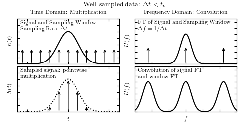
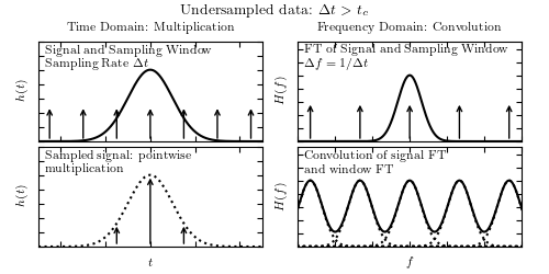
A visualization of aliasing in the Fourier transform. In each set of four panels, the top-left panel shows a signal and a regular sampling function, the top-right panel shows the Fourier transform of the signal and sampling function, the bottom-left panel shows the sampled data, and the bottom-right panel shows the convolution of the Fourier-space representations (cf. figure 10.2). In the top four panels, the data is well sampled, and there is little to no aliasing. In the bottom panels, the data is not well sampled (the spacing between two data points is larger) which leads to aliasing, as seen in the overlap of the convolved Fourier transforms (figure adapted from Greg05).

Code output:

Python source code:

# Author: Jake VanderPlas
# License: BSD
#   The figure produced by this code is published in the textbook
#   "Statistics, Data Mining, and Machine Learning in Astronomy" (2013)
#   For more information, see http://astroML.github.com
#   To report a bug or issue, use the following forum:
#    https://groups.google.com/forum/#!forum/astroml-general
import numpy as np
from matplotlib import pyplot as plt

#----------------------------------------------------------------------
# This function adjusts matplotlib settings for a uniform feel in the textbook.
# Note that with usetex=True, fonts are rendered with LaTeX.  This may
# result in an error if LaTeX is not installed on your system.  In that case,
# you can set usetex to False.
if "setup_text_plots" not in globals():
    from astroML.plotting import setup_text_plots
setup_text_plots(fontsize=8, usetex=True)


def gaussian(x, a=1.0):
    return np.exp(-0.5 * (x / a) ** 2)


def gaussian_FT(f, a=1.0):
    return np.sqrt(2 * np.pi * a ** 2) * np.exp(-2 * (np.pi * a * f) ** 2)

#------------------------------------------------------------
# Define our terms
a = 1.0
t = np.linspace(-5, 5, 1000)
h = gaussian(t, a)

f = np.linspace(-2, 2, 1000)
H = gaussian_FT(f, a)


#------------------------------------------------------------
# Two plots: one well-sampled, one over-sampled
N = 12

for dt in (0.9, 1.5):
    # define time-space sampling
    t_sample = dt * (np.arange(N) - N / 2)
    h_sample = gaussian(t_sample, a)

    # Fourier transform of time-space sampling
    df = 1. / dt
    f_sample = df * (np.arange(N) - N / 2)

    # Plot the results
    fig = plt.figure(figsize=(5, 2.5))
    fig.subplots_adjust(left=0.07, right=0.95, wspace=0.16,
                        bottom=0.1, top=0.85, hspace=0.05)

    # First plot: sampled time-series
    ax = fig.add_subplot(221)
    ax.plot(t, h, '-k')

    for ts in t_sample:
        ax.annotate('', (ts, 0.5), (ts, 0), ha='center', va='center',
                    arrowprops=dict(arrowstyle='->'))
    ax.text(0.03, 0.95,
            ("Signal and Sampling Window\n" +
             r"Sampling Rate $\Delta t$"),
            ha='left', va='top', transform=ax.transAxes)
    ax.set_ylabel('$h(t)$')
    ax.set_xlim(-5, 5)
    ax.set_ylim(0, 1.4)
    ax.xaxis.set_major_formatter(plt.NullFormatter())
    ax.yaxis.set_major_formatter(plt.NullFormatter())
    ax.set_title('Time Domain: Multiplication')

    # second plot: frequency space
    ax = fig.add_subplot(222)
    ax.plot(f, H, '-k')
    for fs in f_sample:
        ax.annotate('', (fs, 1.5), (fs, 0), ha='center', va='center',
                    arrowprops=dict(arrowstyle='->'))
    ax.text(0.03, 0.95,
            ("FT of Signal and Sampling Window\n" +
             r"$\Delta f = 1 / \Delta t$"),
            ha='left', va='top', transform=ax.transAxes)
    ax.set_ylabel('$H(f)$')
    ax.set_xlim(-1.5, 1.5)
    ax.set_ylim(0, 3.8)
    ax.xaxis.set_major_formatter(plt.NullFormatter())
    ax.yaxis.set_major_formatter(plt.NullFormatter())
    ax.set_title('Frequency Domain: Convolution')

    # third plot: windowed function
    ax = fig.add_subplot(223)
    for (ts, hs) in zip(t_sample, h_sample):
        if hs < 0.1:
            continue
        ax.annotate('', (ts, hs), (ts, 0), ha='center', va='center',
                    arrowprops=dict(arrowstyle='->'))
    ax.plot(t, h, ':k')
    ax.text(0.03, 0.95, "Sampled signal: pointwise\nmultiplication",
            ha='left', va='top', transform=ax.transAxes)
    ax.set_xlabel('$t$')
    ax.set_ylabel('$h(t)$')
    ax.set_xlim(-5, 5)
    ax.set_ylim(0, 1.4)
    ax.xaxis.set_major_formatter(plt.NullFormatter())
    ax.yaxis.set_major_formatter(plt.NullFormatter())

    # fourth plot: convolved PSD
    ax = fig.add_subplot(224)
    window = np.array([gaussian_FT(f - fs, a) for fs in f_sample])
    ax.plot(f, window.sum(0), '-k')
    if dt > 1:
        ax.plot(f, window.T, ':k')
    ax.text(0.03, 0.95, "Convolution of signal FT\nand window FT",
            ha='left', va='top', transform=ax.transAxes)
    ax.set_xlabel('$f$')
    ax.set_ylabel('$H(f)$')
    ax.set_xlim(-1.5, 1.5)
    ax.set_ylim(0, 3.8)
    ax.xaxis.set_major_formatter(plt.NullFormatter())
    ax.yaxis.set_major_formatter(plt.NullFormatter())

    if dt > 1:
        fig.suptitle(r"Undersampled data: $\Delta t > t_c$")
    else:
        fig.suptitle(r"Well-sampled data: $\Delta t < t_c$")

plt.show()

[download source: fig_FFT_aliasing.py]